Code
pacman::p_load(olsrr, ggpubr, sf, sfdep, spdep, GWmodel, tmap, tidyverse, gtsummary, httr, jsonlite, rvest, SpatialML)Housing is one of the most basic and essential need for everyone. In Singapore, public housing plays a critical role in meeting the housing needs of the population. One common way of acquiring public housing in Singapore is through the resale market. Many Singaporeans choose to purchase resale HDB flats because of their affordability and relatively short waiting time compared to new flats. As such, the resale market is a critical component of the overall public housing market in Singapore.
The cost of housing is a significant expense for most individuals and families. It is also a major investment for people. As such, understanding the factors that affect the resale prices is important for individuals to make informed decisions when making a purchase. There are many factors influencing the price of housing, whether it be the condition of the economy in general, structural factors (variables related to the property itself), or locational factors (variables related to the positioning of the HDB units).
This project aims to build predictive models of housing resale prices. Two types of models will be explored: conventional OLS regression and geographically-weighted regression.
The R packages used in this project are:
oslrr: for analysing ordinary least squares regression models
ggpubr: for creating production-ready ggplot2 graphs
sf: for importing, managing, and processing geospatial data.
sfdep & spdep: for analysing spatial dependencies
GWmodel: for calibrating geographically-weighted models
tmap: creating thematic maps
tidyverse: a family of other R packages for performing data science tasks such as importing, wrangling, and visualising data.
gtsummary: for creating publication-ready summary tables
httr: for making HTTP requests (used for retrieving information from OneMap API)
jsonlite: for processing JSON format into R data types
rvest: for performing web-scraping (used to scrape the data of the top primary schools)
pacman::p_load(olsrr, ggpubr, sf, sfdep, spdep, GWmodel, tmap, tidyverse, gtsummary, httr, jsonlite, rvest, SpatialML)We will be using a number of geospatial data as independent locational factors to predict HDB resale prices. The datasets used are:
From data.gov.sg:
Location of Hawker Centres
Location of Eldercare centres
Location of Parks
From dataportal.asia (also taken from data.gov.sg):
Location of Childcare centres
Location of Supermarkets
Location of Pre-schools
Location of Kindergartens
From LTA Data Mall:
Location of Bus Stops - 2023
Location of MRT Stations exit
sf_hawker_centres <- st_read("data/geospatial/hawker-centres-kml.kml") %>%
st_transform(3414)
sf_eldercare <- st_read(dsn = "data/geospatial/Eldercare", layer = "ELDERCARE") %>%
st_transform(3414)
sf_parks <- st_read(dsn = "data/geospatial/parks.kml") %>%
st_transform(3414)
sf_childcare <- st_read(dsn = "data/geospatial/childcare.geojson") %>%
st_transform(3414)
sf_supermarkets <- st_read(dsn = "data/geospatial/supermarkets.kml") %>%
st_transform(3414)
sf_preschools <- st_read(dsn = "data/geospatial/preschools-location.kml") %>%
st_transform(3414)
sf_kindergartens <- st_read(dsn = "data/geospatial/kindergartens.kml") %>%
st_transform(3414)
sf_bus_stop <- st_read(dsn = "data/geospatial/BusStop_Feb2023", layer = "BusStop") %>%
st_transform(3414)
sf_mrt <- st_read(dsn = "data/geospatial/TrainStationExit", layer = "Train_Station_Exit_Layer") %>%
st_transform(3414)Additionally, we need the geospatial polygon data for Singapore’s region. For this, we use Master Plan 2019 Subzone Boundary, which contains the geographical boundary of Singapore at the planning subzone level. This particular version of data was provided by Prof. Kam Tin Seong.
mpsz <- st_read(dsn="data/geospatial/MPSZ-2019", layer="MPSZ-2019") %>%
st_transform(3414)Some of the locational factors are not in the form of geospatial data. Rather, they are in the form of CSVs with coordinates. Those datasets are:
Primary Schools (taken from data.world from Hui Xiang Chua)
Singapore Mall Coordinates (taken from Mall SVY21 Coordinates Web Scraper)
We will convert the coordinate data to sf format by using st_as_sf(), and st_transform().
sf_malls <- read_csv("data/aspatial/mall_coordinates_updated.csv") %>%
dplyr::select(c("name", "longitude", "latitude")) %>%
st_as_sf(coords=c("longitude", "latitude"), crs=4326) %>%
st_transform(3414)
sf_primary_schools <- read_csv("data/aspatial/primaryschoolsg.csv") %>%
dplyr::select(c(0:8)) %>%
st_as_sf(coords=c("Longitude", "Latitude"), crs=4326) %>%
st_transform(3414)Most importantly, our core dataset is the HDB Resale Flat Prices provided by data.gov.sg. The distribution of housing prices are dependent on sub-markets. For instance, 2-Room flats and 3-Room flats will have different price distributions, with 3-Room flats generally being higher. In this study, we will be focusing on 3-Room flats.
Additionally, we will only be looking at 1 January 2021 to 31 December 2022 for train data and January-February 2023 for test data. For now, we will import them into one dataframe to make preprocessing easier.
hdb_resale <- read_csv("data/aspatial/resale-flat-prices.csv") %>%
filter(month >= "2021-01" & month <= "2023-02",
flat_type == "3 ROOM")For all the locational factors, we want them to be in the format of spatial points. Therefore, let’s check if any of them are not in the form of points!
To do that, we create a utility function that prints out the name of the object if its geometry type does not match the one we want.
check_geometry_type <- function(sf_obj, desired_geometry) {
if(st_geometry_type(sf_obj, by_geometry = FALSE) != desired_geometry) {
print(deparse(substitute(sf_obj))) # print name of object
}
}check_geometry_type(sf_bus_stop, "POINT")
check_geometry_type(sf_childcare, "POINT")
check_geometry_type(sf_eldercare, "POINT")
check_geometry_type(sf_hawker_centres, "POINT")
check_geometry_type(sf_kindergartens, "POINT")
check_geometry_type(sf_malls, "POINT")
check_geometry_type(sf_parks, "POINT")
check_geometry_type(sf_preschools, "POINT")
check_geometry_type(sf_primary_schools, "POINT")
check_geometry_type(sf_supermarkets, "POINT")
check_geometry_type(sf_mrt, "POINT")
check_geometry_type(mpsz, "MULTIPOLYGON")It seems that all of the geospatial data is in the geometry type we expect them to be.
As we saw with the MRT stations data, sometimes, we might encounter invalid geometries. To err on the side of caution, it’s good practice to check all the geospatial data for such cases.
Again, for convenience, we define a utility function to check the validity of geometries and print out the names of objects that are invalid.
check_geometry_validity <- function(sf_obj) {
if(length(which(st_is_valid(sf_obj) == FALSE |
is.na(st_is_valid(sf_obj)))) > 0) {
print(deparse(substitute(sf_obj))) # print name of object
}
}# Check the locational factors
check_geometry_validity(sf_bus_stop)
check_geometry_validity(sf_childcare)
check_geometry_validity(sf_eldercare)
check_geometry_validity(sf_hawker_centres)
check_geometry_validity(sf_kindergartens)
check_geometry_validity(sf_malls)
check_geometry_validity(sf_parks)
check_geometry_validity(sf_preschools)
check_geometry_validity(sf_primary_schools)
check_geometry_validity(sf_supermarkets)
check_geometry_validity(sf_mrt)
# Check the planning subzone boundaries data
check_geometry_validity(mpsz)[1] "mpsz"It seems that there is a problem with the Subzone Boundaries data. Let’s fix it!
mpsz <- st_make_valid(mpsz)
check_geometry_validity(mpsz)In Singapore, distance affects priority admission to primary schools. Hence, for families with children or expecting to have children, they will likely be concerned about the proximity of their housing unit to good primary schools.
Referring to salary.sg’s 2022 primary school ranking, we can extract the top 20 primary schools into a separate dataframe.
To automate this process, we can use rvest package to scrape the data from the webpage! In doing so, we must inspect the structure of the HTML page and extract only the relevant information (in our case, the ordered list element of the page under the post ID 33132).
primary_schools_ranking <- read_html("https://www.salary.sg/2022/best-primary-schools-2022-by-popularity/") %>%
html_nodes(xpath = paste('//*[@id="post-33132"]/div[3]/div/div/ol/li') ) %>%
html_text() %>%
sapply(gsub, pattern=" – .*", replacement="") %>%
sapply(gsub, pattern=" Section)", replacement=")") %>%
sapply(gsub, pattern="’", replacement="'") %>%
sapply(str_remove_all, pattern="[^A-z|0-9|[:punct:]|\\s]") %>%
unname()
primary_schools_ranking <- primary_schools_ranking[0:20]length(primary_schools_ranking)[1] 20primary_schools_ranking [1] "Methodist Girls' School (Primary)"
[2] "Catholic High School (Primary)"
[3] "Tao Nan School"
[4] "Pei Hwa Presbyterian Primary School"
[5] "Holy Innocents' Primary School"
[6] "Nan Hua Primary School"
[7] "CHIJ St. Nicholas Girls' School (Primary)"
[8] "Admiralty Primary School"
[9] "St. Hilda's Primary School"
[10] "Ai Tong School"
[11] "Anglo-Chinese School (Junior)"
[12] "Chongfu School"
[13] "St. Joseph's Institution Junior"
[14] "Anglo-Chinese School (Primary)"
[15] "Singapore Chinese Girls' Primary School"
[16] "Nanyang Primary School"
[17] "South View Primary School"
[18] "Pei Chun Public School"
[19] "Kong Hwa School"
[20] "Rosyth School" Now, we can filter out based on the names.
sf_good_primary_schools <- sf_primary_schools %>%
filter(Name %in% primary_schools_ranking)
nrow(sf_good_primary_schools)[1] 19It seems that we are missing one primary school. Checking to see which name from the ranking list is missing from the data frame:
unique(primary_schools_ranking[!(primary_schools_ranking %in% sf_good_primary_schools$Name)])[1] "CHIJ St. Nicholas Girls' School (Primary)"In the original sf_primary_schools dataframe, it is called “CHIJ St. Nicholas Girls’ School”. Therefore, let us manually add this record to sf_good_primary_schools.
sf_good_primary_schools <- sf_good_primary_schools %>%
rbind(sf_primary_schools %>% filter(Name == "CHIJ St. Nicholas Girls' School"))nrow(sf_good_primary_schools)[1] 20glimpse(hdb_resale)Rows: 13,780
Columns: 11
$ month <chr> "2021-01", "2021-01", "2021-01", "2021-01", "2021-…
$ town <chr> "ANG MO KIO", "ANG MO KIO", "ANG MO KIO", "ANG MO …
$ flat_type <chr> "3 ROOM", "3 ROOM", "3 ROOM", "3 ROOM", "3 ROOM", …
$ block <chr> "331", "534", "561", "170", "463", "542", "170", "…
$ street_name <chr> "ANG MO KIO AVE 1", "ANG MO KIO AVE 10", "ANG MO K…
$ storey_range <chr> "04 TO 06", "04 TO 06", "01 TO 03", "07 TO 09", "0…
$ floor_area_sqm <dbl> 68, 68, 68, 60, 68, 68, 60, 73, 67, 67, 68, 68, 73…
$ flat_model <chr> "New Generation", "New Generation", "New Generatio…
$ lease_commence_date <dbl> 1981, 1980, 1980, 1986, 1980, 1981, 1986, 1976, 19…
$ remaining_lease <chr> "59 years", "58 years 02 months", "58 years 01 mon…
$ resale_price <dbl> 260000, 265000, 265000, 268000, 268000, 270000, 27…As we can observe, there are no columns indicating the longitude and latitude coordinates of the HDB. This is troublesome, seeing that for our geospatial analysis, we need the exact location of the units. Fortunately, Singapore has the OneMap API, which allows you to query for coordinates given an address.
Using the httr package, we can invoke HTTP requests. The OneMap API exposes a /search endpoint, which allows you to search for the longitude and latitude of a given address. We can create a function to invoke this API with the addresses of the HDB flats and return the coordinates.
get_onemap_coords <- function(address) {
r <- httr::GET('https://developers.onemap.sg/commonapi/search?',
query=list(searchVal=address,
returnGeom='Y',
getAddrDetails='Y',
pageNum = '1'))
data <- fromJSON(rawToChar(r$content))
res <- data$results %>%
head(res, n=1) %>%
mutate(SEARCH_KEY = address, .before = 1)
return(res)
}In our data, we only have the block number and street name. Let’s create a column with the full address that we can pass into our get_onemap_coords() function!
hdb_resale <- hdb_resale %>%
mutate(joined_address = paste(hdb_resale$block, hdb_resale$street_name))Afterwards, we can create a new dataframe from the results of our get_onemap_coords() function. To save computational time, we can just query for unique addresses.
hdb_onemap_coords <- unique(hdb_resale$joined_address) %>%
lapply(get_onemap_coords) %>%
Reduce(full_join, .) %>%
select(c("SEARCH_KEY", "BLK_NO", "ROAD_NAME", "ADDRESS", "POSTAL", "LATITUDE", "LONGITUDE"))We can save it into an RDS file format for future use.
write_rds(hdb_onemap_coords, "data/rds/hdb_onemap_coords.rds")Afterwards, we can perform a left join of the coordinates to our original data.
hdb_onemap_coords <- read_rds("data/rds/hdb_onemap_coords.rds")
hdb_resale_coords <- left_join(hdb_resale, hdb_onemap_coords, multiple="all", by=c("joined_address" = "SEARCH_KEY"))Now that we have the longitude and latitude, we can transform it into an sf dataframe.
sf_hdb_resale_coords <- hdb_resale_coords %>%
st_as_sf(coords=c("LONGITUDE", "LATITUDE"), crs=4326) %>%
st_transform(3414)For our analysis, we will be using these structural factors:
floor_area_sqm: area of the unit
storey_range: floor level of the unit
remaining_lease: remaining lease period
Age of the unit (to be derived from lease_commence_date)
glimpse(hdb_resale_coords)Rows: 13,780
Columns: 18
$ month <chr> "2021-01", "2021-01", "2021-01", "2021-01", "2021-…
$ town <chr> "ANG MO KIO", "ANG MO KIO", "ANG MO KIO", "ANG MO …
$ flat_type <chr> "3 ROOM", "3 ROOM", "3 ROOM", "3 ROOM", "3 ROOM", …
$ block <chr> "331", "534", "561", "170", "463", "542", "170", "…
$ street_name <chr> "ANG MO KIO AVE 1", "ANG MO KIO AVE 10", "ANG MO K…
$ storey_range <chr> "04 TO 06", "04 TO 06", "01 TO 03", "07 TO 09", "0…
$ floor_area_sqm <dbl> 68, 68, 68, 60, 68, 68, 60, 73, 67, 67, 68, 68, 73…
$ flat_model <chr> "New Generation", "New Generation", "New Generatio…
$ lease_commence_date <dbl> 1981, 1980, 1980, 1986, 1980, 1981, 1986, 1976, 19…
$ remaining_lease <chr> "59 years", "58 years 02 months", "58 years 01 mon…
$ resale_price <dbl> 260000, 265000, 265000, 268000, 268000, 270000, 27…
$ joined_address <chr> "331 ANG MO KIO AVE 1", "534 ANG MO KIO AVE 10", "…
$ BLK_NO <chr> "331", "534", "561", "170", "463", "542", "170", "…
$ ROAD_NAME <chr> "ANG MO KIO AVENUE 1", "ANG MO KIO AVENUE 10", "AN…
$ ADDRESS <chr> "331 ANG MO KIO AVENUE 1 TECK GHEE VIEW SINGAPORE …
$ POSTAL <chr> "560331", "560534", "560561", "560170", "NIL", "56…
$ LATITUDE <chr> "1.36211140665392", "1.37405846295585", "1.3705776…
$ LONGITUDE <chr> "103.850766473498", "103.854168170426", "103.85785…If we look at our HDB resale data, we can see that some of them are actually categorical variables, such as storey_range and remaining_lease. Categorical variables need some special treatment, as they cannot be input into a regression model as they are. Hence, we need to transform them into an appropriate format. Normally, this is done through one-hot encoding, in which we create dummy columns of 0’s and 1’s according to its category.
However, categorical variables might also be ordered. From a glance, we can suspect that this is the case with storey_range.
unique(sf_hdb_resale_coords$storey_range) [1] "04 TO 06" "01 TO 03" "07 TO 09" "10 TO 12" "13 TO 15" "28 TO 30"
[7] "19 TO 21" "16 TO 18" "25 TO 27" "22 TO 24" "34 TO 36" "40 TO 42"
[13] "31 TO 33" "37 TO 39" "46 TO 48" "43 TO 45"Whereas remaining_lease is in the form of character strings that denote number of years and months left.
Hence, it might be more useful for us to convert them into numeric values!
Before we convert storey_range into a numeric value, we need to decide whether we should convert it to one-hot encoding or ordinal numbers.
This is because we will be predicting resale prices using linear regression. Hence, the choice of encoding is important here because it will make a difference in how the calculations are done.
predicted_housing_price = w1 * (1 or 0 if storey_range = “01 TO 03”) + w2 * (1 or 0 if storey_range = “04 TO 06”) + ….
This implies that each category are treated individually.
predicted_housing_price = w * (ordinally encoded storey_range, e.g. “01 TO 03” = 1, “04 TO 06” = 2, …)
This implies that the higher the storey where the unit is located, the higher its resale price should be.
To get an idea, we can briefly visualise the mean resale price for each category.
ggplot(sf_hdb_resale_coords %>%
group_by(storey_range) %>%
summarise(mean_price = mean(resale_price)),
aes(x=storey_range, y=mean_price)) +
geom_col(fill="light coral") +
labs(title = "Mean Resale Price vs. Storey Range",
x = "Storey Range",
y = "Mean Resale Price") +
theme(axis.text.x = element_text(angle=90))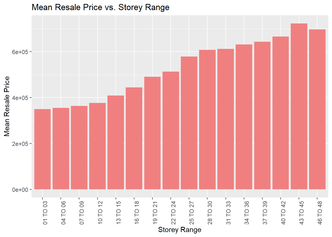
From this, we can suspect that there might be a positive linear correlation between the resale price and the storey range. Hence, it will be a good idea to encode it into ordinal numbers to capture this relationship.
In R, we have a data type called factors, which allows us to associate an order to character values. We can create an ordered factor using the ordered() function.
# Levels of the ordered factor
levels(ordered(sf_hdb_resale_coords$storey_range)) [1] "01 TO 03" "04 TO 06" "07 TO 09" "10 TO 12" "13 TO 15" "16 TO 18"
[7] "19 TO 21" "22 TO 24" "25 TO 27" "28 TO 30" "31 TO 33" "34 TO 36"
[13] "37 TO 39" "40 TO 42" "43 TO 45" "46 TO 48"Using the mutate() function of dplyr, we can add this encoding as another column to sf_hdb_resale_coords.
sf_hdb_resale_coords <- sf_hdb_resale_coords %>%
mutate(storey_range_encoded = as.numeric(ordered(storey_range)))There are two different ways remaining_lease is represented: “xx years yy months” or “xx years”. For simplicity, we will convert the values into number of months.
Let’s create a utility function to calculate the number of months given that format. We will use the str_split() function to split the words and calculate the total number of months.
calculate_months <- function(lease_string) {
str_list <- str_split(lease_string, " ") %>% unlist()
if (length(str_list) > 2) {
year <- as.numeric(str_list[1])
month <- as.numeric(str_list[3])
return(year * 12 + month)
} else {
year <- as.numeric(str_list[1])
return(year * 12)
}
}Now, we can create a new column called remaining_lease_months! We use purrr’s map_int() function to apply the scalar function to every element in the remaining_lease column.
sf_hdb_resale_coords <- sf_hdb_resale_coords %>%
mutate(remaining_lease_months = map_int(remaining_lease, calculate_months))Derive age of the unit
We will derive the age of the unit by subtracting the year of the resale (taken from the month column) with the lease_commence_date. The age of the unit will be in years.
sf_hdb_resale_coords <- sf_hdb_resale_coords %>%
mutate(unit_age = as.numeric(substring(month, 0, 4)) - lease_commence_date)Now, we can incorporate the locational factors into the HDB resale data. We are interested in:
Proximity to certain facilities
Count of facilities within a specified radius
We can get the proximity to the nearest facility by calculating a matrix of distances using sf’s st_distance() function. We calculate the lowest row-wise value of the matrix for each HDB unit in kilometers, and append it as a column to the dataframe.
get_proximity <- function(origin_df, dest_df, col_name) {
# creates a matrix of distances
dist_matrix <- st_distance(origin_df, dest_df)
# Get the lowest distance for every facility
origin_df <- origin_df %>%
mutate(PROX = apply(dist_matrix, 1, min) / 1000) %>%
rename(!!col_name := PROX)
# use the !! operator to "unquote" the variable
# and := to substitute
return(origin_df)
}One of the locational factors of interest that we want to take into account is the proximity to Singapore’s CBD. This encompasses the Downtown Core planning area. To get the proximity, we can simply check against the centroid of the Downtown Core area.
# Extract Downtown core
downtown_core <- mpsz %>%
filter(PLN_AREA_N == "DOWNTOWN CORE") %>%
st_combine()
# Get Centroid
downtown_core_centroid <- downtown_core %>%
st_centroid()We can view the centroid of the Downtown Core.
tmap_mode("view")
tm_shape(downtown_core) +
tm_fill(col = "turquoise", alpha=0.5) +
tm_borders(alpha=0.5) +
tm_shape(downtown_core_centroid) +
tm_bubbles(col = "blue") +
tmap_options(check.and.fix=TRUE) +
tm_view(set.zoom.limits=c(13,15))Using our get_proximity() utility function, we can calculate the proximity to the CBD.
sf_hdb_resale_coords <- sf_hdb_resale_coords %>%
get_proximity(downtown_core_centroid, "PROX_CBD")We can repeat this process as it is with the other locational factors.
sf_hdb_resale_coords <- sf_hdb_resale_coords %>%
get_proximity(sf_eldercare, "PROX_ELDERCARE") %>%
get_proximity(sf_hawker_centres, "PROX_HAWKER_CENTRE") %>%
get_proximity(sf_mrt, "PROX_MRT") %>%
get_proximity(sf_parks, "PROX_PARK") %>%
get_proximity(sf_malls, "PROX_MALL") %>%
get_proximity(sf_supermarkets, "PROX_SUPERMARKET") %>%
get_proximity(sf_good_primary_schools, "PROX_GOOD_PRIMARY_SCHOOL")For the count of facilities, we are interested in getting:
Number of kindergartens within 350m
Number of childcare centres within 350m
Number of bus stops within 350m
Number of primary schools within 1km
To do this, we can again create a matrix of distances with st_distance(). Afterwards, we can find the count of values within each row of the matrix that falls within the specified distance in meters. This value will be appended to the dataframe as a new column.
get_count_within <- function(origin_df, dest_df, threshold_dist, col_name){
# creates a matrix of distances
dist_matrix <- st_distance(origin_df, dest_df)
# count the number of location_factors within threshold_dist and create new data frame
origin_df <- origin_df %>%
mutate(
WITHIN_DT = apply(dist_matrix, 1, function(x) sum(x <= threshold_dist))
) %>%
rename(!!col_name := WITHIN_DT)
# Return df
return(origin_df)
}Now, we can calculate the number of facilities within the radius.
sf_hdb_resale_coords <- sf_hdb_resale_coords %>%
get_count_within(sf_kindergartens, 350, "WITHIN_350M_KINDERGARTEN") %>%
get_count_within(sf_childcare, 350, "WITHIN_350M_CHILDCARE") %>%
get_count_within(sf_bus_stop, 350, "WITHIN_350M_BUS") %>%
get_count_within(sf_primary_schools, 1000, "WITHIN_1KM_PRIMARY_SCHOOL")Now that we’re done with all the preprocessing, we should save our data for future use, so that we don’t have to go through the whole preprocessing steps again!
First of all, we should only select columns relevant to our analysis.
sf_hdb_resale_factors <- sf_hdb_resale_coords %>%
dplyr::select(c("month", "resale_price", "floor_area_sqm", "flat_type",
"storey_range_encoded", "remaining_lease_months", "unit_age",
"PROX_CBD", "PROX_ELDERCARE", "PROX_HAWKER_CENTRE",
"PROX_MRT", "PROX_PARK", "PROX_MALL", "PROX_SUPERMARKET",
"PROX_GOOD_PRIMARY_SCHOOL", "WITHIN_350M_KINDERGARTEN",
"WITHIN_350M_CHILDCARE", "WITHIN_350M_BUS",
"WITHIN_1KM_PRIMARY_SCHOOL"))We can then save it into RDS format,
write_rds(sf_hdb_resale_factors, "data/rds/hdb_resale_factors.rds")and retrieve it when we need it!
sf_hdb_resale_factors <- read_rds("data/rds/hdb_resale_factors.rds")We can view the locational factors in the form of interactive maps. Use the layer panel (the button on the left side of the interactive map underneath the zoom buttons) to toggle which things you want to view.
We can divide the locational factors into 3 categories: Care (i.e. Childcare/Eldercare) & Education (i.e. Kindegrartens, Preschools), General Amenities (i.e. Hawker Centres, Shopping Malls, Parks, Supermarkets), and Transportation (i.e. MRT Stations and Bus Stops).
tmap_mode('view')
tm_shape(sf_eldercare) +
tm_dots(col="blue", alpha=0.4, id="NAME") +
tm_shape(sf_childcare) +
tm_dots(col="red", alpha=0.4) +
tm_shape(sf_kindergartens) +
tm_dots(col="green", alpha=0.4) +
tm_shape(sf_preschools) +
tm_dots(col="purple", alpha=0.4) +
tm_shape(sf_primary_schools) +
tm_dots(col="yellow", alpha=0.4, id="Name") +
tm_view(set.zoom.limits=c(11,15))tmap_mode('view')
tm_shape(sf_hawker_centres) +
tm_dots(col="blue", alpha=0.4) +
tm_shape(sf_malls) +
tm_dots(col="purple", alpha=0.4, id="name") +
tm_shape(sf_parks) +
tm_dots(col="green", alpha=0.4, id="Name") +
tm_shape(sf_supermarkets) +
tm_dots(col="turquoise", alpha=0.4) +
tm_view(set.zoom.limits=c(11,15))tmap_mode('view')
tm_shape(sf_bus_stop) +
tm_dots(col="blue", id="LOC_DESC", alpha=0.4) +
tm_shape(sf_mrt) +
tm_dots(col="yellow", id="STN_NAM_DE", alpha=0.4) +
tm_view(set.zoom.limits=c(11,15)) We can visualise the distribution of HDB resale prices using histograms.
options(scipen = 999)
ggplot(data=sf_hdb_resale_factors, aes(x=`resale_price`)) +
geom_histogram(bins=20, color="black", fill="light blue") +
labs(title = "Distribution of Resale Prices",
x = "Resale Prices",
y = "Frequency") +
scale_x_continuous(labels = scales::comma)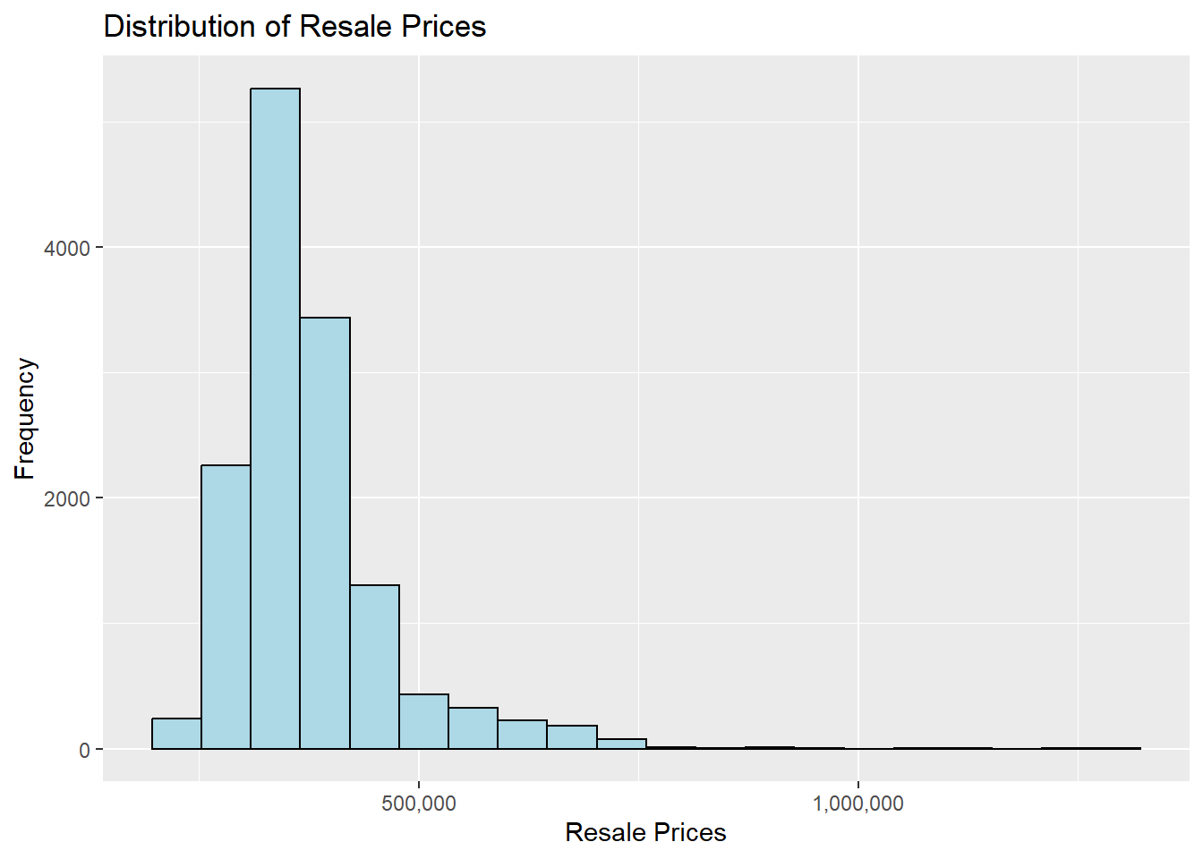
We can see that the distribution of the prices seem to be right-skewed. We can normalise this using a log transformation. Using dplyr’s mutate() function, we can add a column of log-normalised resale price values.
sf_hdb_resale_factors <- sf_hdb_resale_factors %>%
mutate(`resale_price_log` = log(resale_price))ggplot(data=sf_hdb_resale_factors, aes(x=`resale_price_log`)) +
geom_histogram(bins=20, color="black", fill="light blue") +
labs(title = "Distribution of Log(Resale Prices)",
x = "Log(Resale Prices)",
y = "Frequency")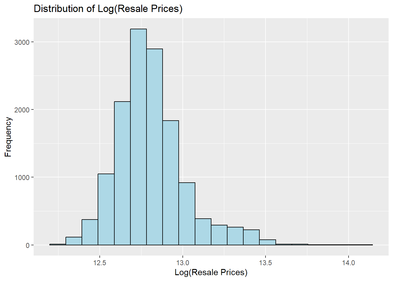
We can see that the post-log-normalised data is less skewed. However, for our analysis, we will still be using the original prices.
Let’s also view the distribution of the structural factors and the locational factors over the whole market.
plot_floor_area <- ggplot(data=sf_hdb_resale_factors, aes(x=floor_area_sqm)) +
geom_histogram(bins=20, color="black", fill="light green") +
labs(x = "Area of unit",
y = "Frequency")
plot_storey <- ggplot(data=sf_hdb_resale_factors, aes(x=storey_range_encoded)) +
geom_histogram(bins=20, color="black", fill="light green") +
labs(x = "Storey group",
y = "Frequency")
plot_unit_age <- ggplot(data=sf_hdb_resale_factors, aes(x=unit_age)) +
geom_histogram(bins=20, color="black", fill="light green") +
labs(x = "Age of unit",
y = "Frequency")
plot_remaining_lease_months <- ggplot(data=sf_hdb_resale_factors, aes(x=remaining_lease_months)) +
geom_histogram(bins=20, color="black", fill="light green") +
labs(x = "Remaining lease (mths)",
y = "Frequency")
ggarrange(plot_floor_area, plot_storey, plot_unit_age, plot_remaining_lease_months, ncol = 2, nrow = 2)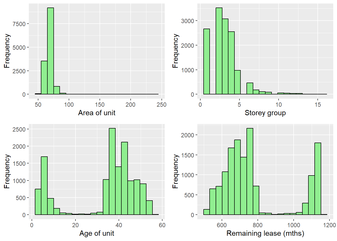
Proximity
plot_PROX_CBD <- ggplot(data=sf_hdb_resale_factors, aes(x=PROX_CBD)) +
geom_histogram(bins=20, color="black", fill="light coral")
plot_PROX_ELDERCARE <- ggplot(data=sf_hdb_resale_factors, aes(x=PROX_ELDERCARE)) +
geom_histogram(bins=20, color="black", fill="light coral")
plot_PROX_HAWKER_CENTRE <- ggplot(data=sf_hdb_resale_factors, aes(x=PROX_HAWKER_CENTRE)) +
geom_histogram(bins=20, color="black", fill="light coral")
plot_PROX_MRT <- ggplot(data=sf_hdb_resale_factors, aes(x=PROX_MRT)) +
geom_histogram(bins=20, color="black", fill="light coral")
plot_PROX_MALL <- ggplot(data=sf_hdb_resale_factors, aes(x=PROX_MALL)) +
geom_histogram(bins=20, color="black", fill="light coral")
plot_PROX_SUPERMARKET <- ggplot(data=sf_hdb_resale_factors, aes(x=PROX_SUPERMARKET)) +
geom_histogram(bins=20, color="black", fill="light coral")
plot_PROX_GOOD_PRIMARY_SCHOOL <- ggplot(data=sf_hdb_resale_factors, aes(x=PROX_GOOD_PRIMARY_SCHOOL)) +
geom_histogram(bins=20, color="black", fill="light coral")
ggarrange(plot_PROX_CBD, plot_PROX_ELDERCARE, plot_PROX_HAWKER_CENTRE,
plot_PROX_MRT, plot_PROX_MALL, plot_PROX_SUPERMARKET,
plot_PROX_GOOD_PRIMARY_SCHOOL, ncol = 2, nrow = 4)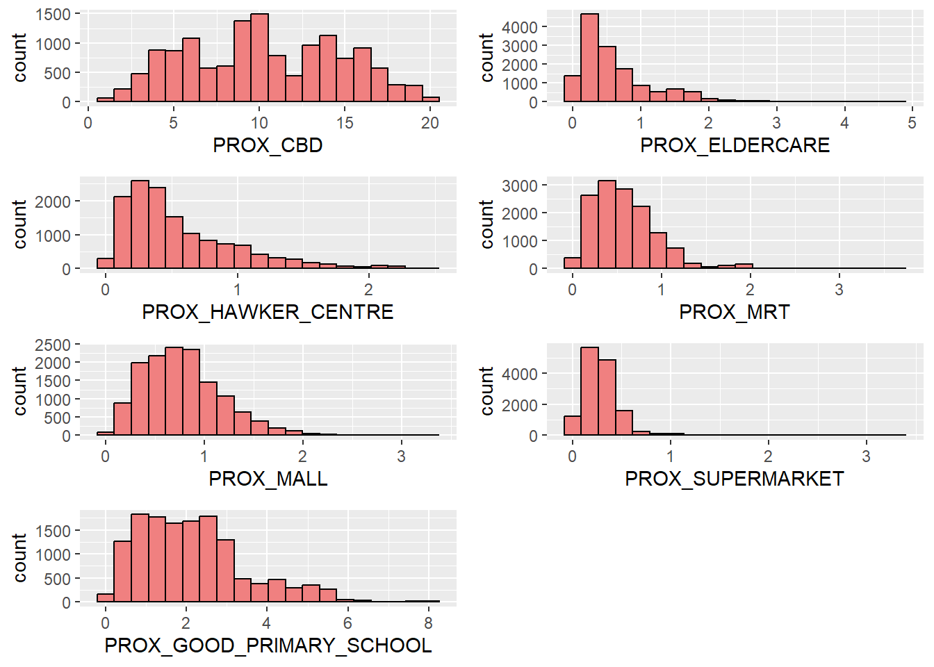
Count within radius
plot_WITHIN_350M_KINDERGARTEN <- ggplot(data=sf_hdb_resale_factors, aes(x=WITHIN_350M_KINDERGARTEN)) +
geom_histogram(bins=20, color="black", fill="plum")
plot_WITHIN_350M_CHILDCARE <- ggplot(data=sf_hdb_resale_factors, aes(x=WITHIN_350M_KINDERGARTEN)) +
geom_histogram(bins=20, color="black", fill="plum")
plot_WITHIN_350M_BUS <- ggplot(data=sf_hdb_resale_factors, aes(x=WITHIN_350M_BUS)) +
geom_histogram(bins=20, color="black", fill="plum")
plot_WITHIN_1KM_PRIMARY_SCHOOL <- ggplot(data=sf_hdb_resale_factors, aes(x=WITHIN_1KM_PRIMARY_SCHOOL)) +
geom_histogram(bins=20, color="black", fill="plum")
ggarrange(plot_WITHIN_350M_KINDERGARTEN, plot_WITHIN_350M_CHILDCARE,
plot_WITHIN_350M_BUS, plot_WITHIN_1KM_PRIMARY_SCHOOL,
ncol = 2, nrow = 2)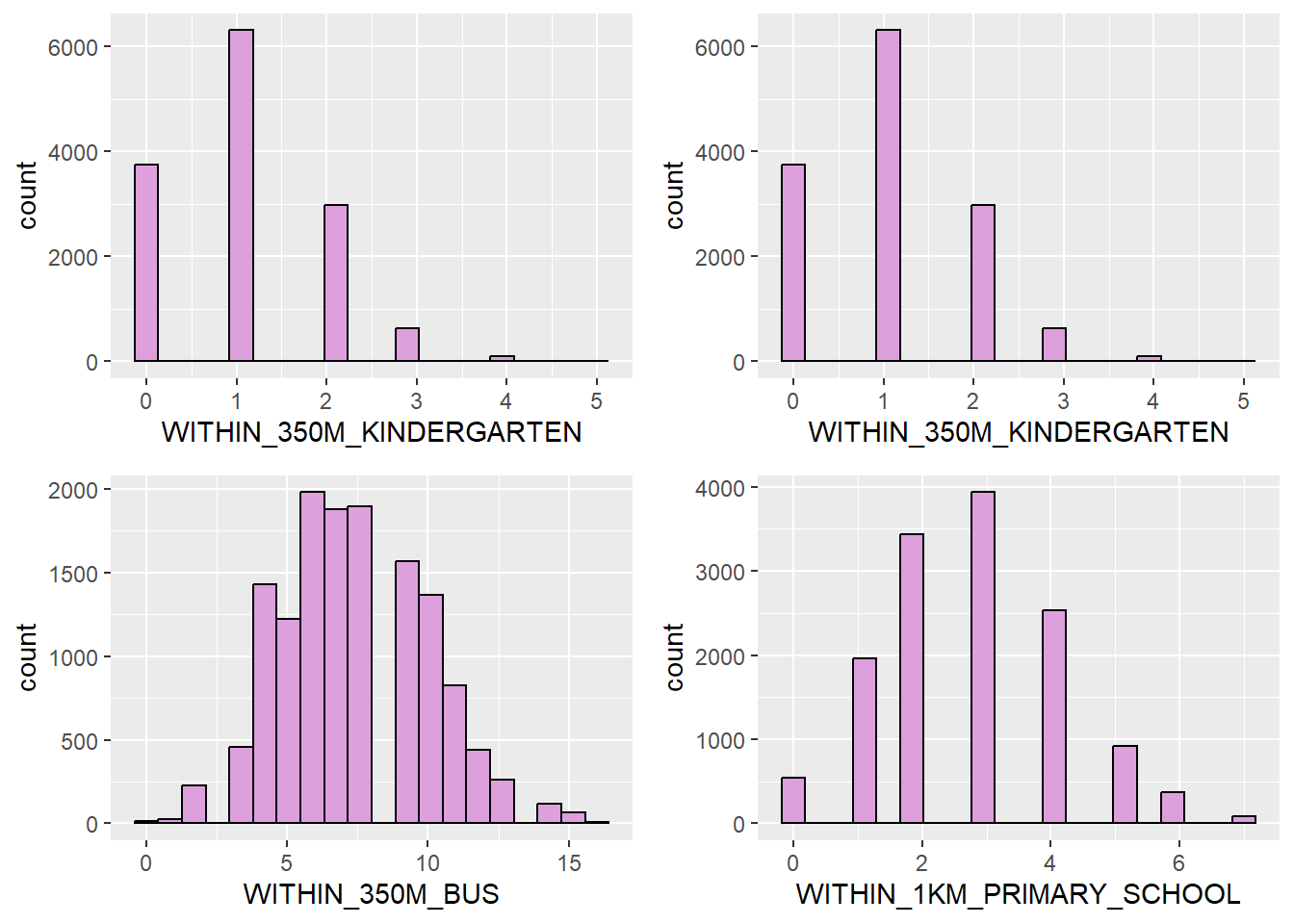
This study is focused on using different predictive models to try to predict the resale price of HDBs given the independent variables. In this study, we will be evaluating the performance of two models: Ordinary Least Squares Multiple Linear Regression (over the entire sample) and Geographically Weighted Random Forest.
Before moving on to the predictive modelling, we need to check if our independent variables are not heavily correlated. Heavily correlated features serve to increase the complexity of the model without adding much information, thus making our model more prone to errors. If there are any heavily correlated features, we need to remove them!
We will use the corrplot package to plot a correlation matrix of our variables.
draw_correlation_plot <- function(sf_df) {
corr_matrix <- sf_df %>%
select(c("floor_area_sqm", 5:20)) %>%
st_drop_geometry() %>%
cor()
return(corrplot::corrplot(corr_matrix, diag = FALSE, order = "AOE", method = "number", type = "full"))
}
draw_correlation_plot(sf_hdb_resale_factors)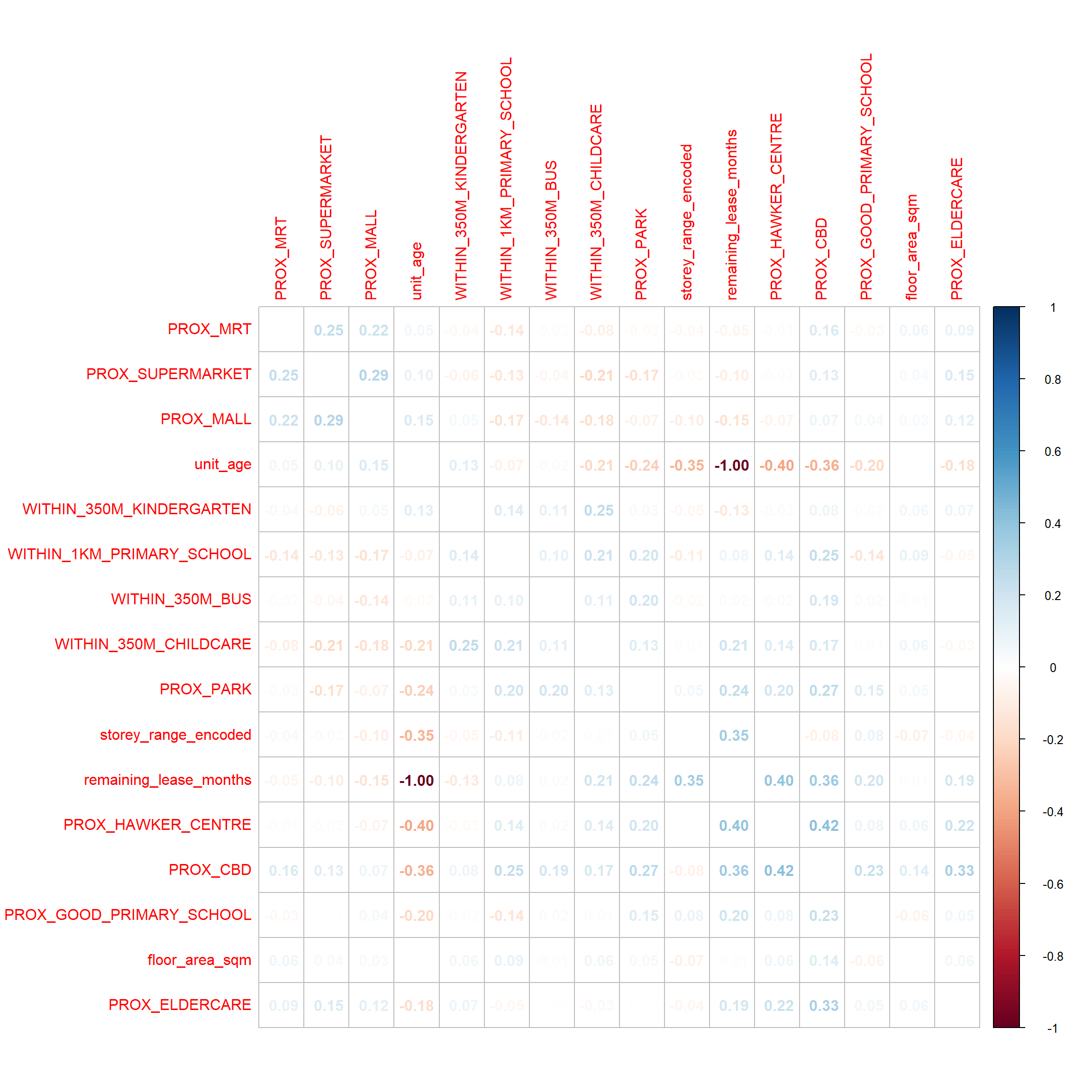
There appears to be a heavy negative correlation between remaining_lease_months and unit_age. This makes sense because the total remaining lease would be inversely proportional to how long the unit has existed. For example, assume that the total length of the lease is 99 years. For a unit built in 1980, its lease period would be until 2079. In the year 2021, the age of the unit would be 41 years (2021 - 1980), while the remaining lease period would be 58 years (2079 - 2021). For the purpose of this study, it would make sense to keep the remaining lease in months. Not only does it provide a more accurate measure of time by taking into account the months, people are likely to be concerned about how long they will be able to own the flat before the lease period is over. This will likely affect their decision to purchase the flat and the price.
sf_hdb_resale_factors <- sf_hdb_resale_factors %>%
dplyr::select(-unit_age)When doing predictive modeling, it is not sufficient to report error metrics on the training data alone. We want to evaluate how well the model generalises to data points that it hasn’t seen before. Despite a low training error, a model might perform badly on new data points due to overfitting (i.e. it fits the training data too well that it is unable to generalise).
As a rule of thumb, to ensure that our evaluation is unbiased, the test set must be kept completely separate from the model training! As such, as mentioned in the Data Import section, we will be taking 1 January 2021 to 31 December 2022 for train data and January-February 2023 for test data.
We will also save them into RDS file format, so that we can load them for future use.
train_data <- sf_hdb_resale_factors %>%
filter(month >= "2021-01" & month <= "2022-12") %>%
write_rds("data/rds/train_data.rds")
test_data <- sf_hdb_resale_factors %>%
filter(month >= "2023-01" & month <= "2023-02") %>%
write_rds("data/rds/test_data.rds")Whenever we want to use the data, we can reload a fresh copy from the RDS file.
train_data <- read_rds("data/rds/train_data.rds")
test_data <- read_rds("data/rds/test_data.rds")We can use stats package’s lm() function to fit a multiple linear regression on our data. Our dependent variable (the value we want to predict) y is resale_price, while our independent variables are all the other columns in sf_hdb_resale_factors.
set.seed(8008)
ols_price_mlr <- lm(resale_price ~ floor_area_sqm +
storey_range_encoded + remaining_lease_months +
PROX_CBD + PROX_ELDERCARE + PROX_HAWKER_CENTRE +
PROX_MRT + PROX_PARK + PROX_MALL +
PROX_SUPERMARKET + PROX_GOOD_PRIMARY_SCHOOL +
WITHIN_350M_KINDERGARTEN +
WITHIN_350M_CHILDCARE + WITHIN_350M_BUS +
WITHIN_1KM_PRIMARY_SCHOOL,
data=train_data)Let’s save the result of this model for future use!
write_rds(ols_price_mlr, "data/model/ols_price_mlr.rds")For the coefficients learned by the model, we set the significance level at 0.05. We can remove any variables that are statistically insignificant (i.e. p-value > 0.05).
ols_price_mlr <- read_rds("data/model/ols_price_mlr.rds")
tbl_regression(ols_price_mlr,
intercept = TRUE) %>%
add_glance_source_note(
label = list(sigma ~ "\U03C3"),
include = c(r.squared, adj.r.squared,
AIC, statistic,
p.value, sigma))| Characteristic | Beta | 95% CI1 | p-value |
|---|---|---|---|
| (Intercept) | -123,016 | -134,212, -111,819 | <0.001 |
| floor_area_sqm | 5,047 | 4,905, 5,189 | <0.001 |
| storey_range_encoded | 10,602 | 10,062, 11,141 | <0.001 |
| remaining_lease_months | 293 | 287, 299 | <0.001 |
| PROX_CBD | -7,485 | -7,757, -7,213 | <0.001 |
| PROX_ELDERCARE | -3,997 | -5,805, -2,190 | <0.001 |
| PROX_HAWKER_CENTRE | -7,476 | -9,917, -5,034 | <0.001 |
| PROX_MRT | -12,468 | -15,066, -9,869 | <0.001 |
| PROX_PARK | -7,259 | -10,006, -4,512 | <0.001 |
| PROX_MALL | -19,369 | -21,833, -16,904 | <0.001 |
| PROX_SUPERMARKET | 24,607 | 19,558, 29,656 | <0.001 |
| PROX_GOOD_PRIMARY_SCHOOL | -752 | -1,470, -35 | 0.040 |
| WITHIN_350M_KINDERGARTEN | 2,476 | 1,356, 3,596 | <0.001 |
| WITHIN_350M_CHILDCARE | -2,257 | -2,862, -1,652 | <0.001 |
| WITHIN_350M_BUS | 1,001 | 644, 1,358 | <0.001 |
| WITHIN_1KM_PRIMARY_SCHOOL | -3,057 | -3,792, -2,321 | <0.001 |
| R² = 0.655; Adjusted R² = 0.654; AIC = 309,250; Statistic = 1,593; p-value = <0.001; σ = 51,245 | |||
| 1 CI = Confidence Interval | |||
However, fortunately, it seems that all of our variables are statistically significant! Let’s view a breakdown of our model’s metrics.
ols_regress(ols_price_mlr) Model Summary
----------------------------------------------------------------------
R 0.809 RMSE 51245.082
R-Squared 0.655 Coef. Var 13.811
Adj. R-Squared 0.654 MSE 2626058446.567
Pred R-Squared 0.654 MAE 38069.849
----------------------------------------------------------------------
RMSE: Root Mean Square Error
MSE: Mean Square Error
MAE: Mean Absolute Error
ANOVA
-----------------------------------------------------------------------------------------
Sum of
Squares DF Mean Square F Sig.
-----------------------------------------------------------------------------------------
Regression 62738198804773.688 15 4182546586984.913 1592.709 0.0000
Residual 33067327959175.605 12592 2626058446.567
Total 95805526763949.297 12607
-----------------------------------------------------------------------------------------
Parameter Estimates
----------------------------------------------------------------------------------------------------------------------
model Beta Std. Error Std. Beta t Sig lower upper
----------------------------------------------------------------------------------------------------------------------
(Intercept) -123015.672 5711.993 -21.536 0.000 -134212.048 -111819.296
floor_area_sqm 5047.072 72.443 0.372 69.670 0.000 4905.073 5189.070
storey_range_encoded 10601.512 275.010 0.225 38.550 0.000 10062.451 11140.574
remaining_lease_months 292.701 3.126 0.642 93.643 0.000 286.574 298.828
PROX_CBD -7485.375 138.738 -0.383 -53.953 0.000 -7757.323 -7213.428
PROX_ELDERCARE -3997.223 922.169 -0.025 -4.335 0.000 -5804.814 -2189.631
PROX_HAWKER_CENTRE -7475.594 1245.579 -0.037 -6.002 0.000 -9917.119 -5034.069
PROX_MRT -12467.857 1325.616 -0.053 -9.405 0.000 -15066.267 -9869.447
PROX_PARK -7259.318 1401.507 -0.030 -5.180 0.000 -10006.484 -4512.151
PROX_MALL -19368.504 1257.172 -0.090 -15.406 0.000 -21832.752 -16904.255
PROX_SUPERMARKET 24607.100 2575.998 0.056 9.552 0.000 19557.752 29656.449
PROX_GOOD_PRIMARY_SCHOOL -752.176 366.021 -0.012 -2.055 0.040 -1469.634 -34.718
WITHIN_350M_KINDERGARTEN 2475.650 571.410 0.024 4.333 0.000 1355.600 3595.701
WITHIN_350M_CHILDCARE -2257.166 308.740 -0.043 -7.311 0.000 -2862.344 -1651.988
WITHIN_350M_BUS 1000.977 182.280 0.030 5.491 0.000 643.681 1358.273
WITHIN_1KM_PRIMARY_SCHOOL -3056.531 375.309 -0.048 -8.144 0.000 -3792.193 -2320.868
----------------------------------------------------------------------------------------------------------------------The R2 and adjusted R2 values are around 0.65, which implies that around 65% of variance is explained by the model. The root mean square error (RMSE) between the training data and the best fit line is 51245.082.
When using the ranger function, we need to first extract the coordinates of the data and drop the geometry column.
coords_train <- st_coordinates(train_data)
coords_test <- st_coordinates(test_data)
train_data <- st_drop_geometry(train_data)
test_data <- st_drop_geometry(test_data)We can save the coordinates to RDS for future use.
write_rds(coords_train, "data/rds/coords_train.rds")
write_rds(coords_test, "data/rds/coords_test.rds")Now, let’s train the random forest using ranger!
set.seed(8008)
rf <- ranger(resale_price ~ floor_area_sqm +
storey_range_encoded + remaining_lease_months +
PROX_CBD + PROX_ELDERCARE + PROX_HAWKER_CENTRE +
PROX_MRT + PROX_PARK + PROX_MALL +
PROX_SUPERMARKET + PROX_GOOD_PRIMARY_SCHOOL +
WITHIN_350M_KINDERGARTEN +
WITHIN_350M_CHILDCARE + WITHIN_350M_BUS +
WITHIN_1KM_PRIMARY_SCHOOL,
data=train_data,
num.trees = 20)
write_rds(rf, "data/model/price_rf.rds")rf <- read_rds("data/model/price_rf.rds")
rfRanger result
Call:
ranger(resale_price ~ floor_area_sqm + storey_range_encoded + remaining_lease_months + PROX_CBD + PROX_ELDERCARE + PROX_HAWKER_CENTRE + PROX_MRT + PROX_PARK + PROX_MALL + PROX_SUPERMARKET + PROX_GOOD_PRIMARY_SCHOOL + WITHIN_350M_KINDERGARTEN + WITHIN_350M_CHILDCARE + WITHIN_350M_BUS + WITHIN_1KM_PRIMARY_SCHOOL, data = train_data, num.trees = 20)
Type: Regression
Number of trees: 20
Sample size: 12608
Number of independent variables: 15
Mtry: 3
Target node size: 5
Variable importance mode: none
Splitrule: variance
OOB prediction error (MSE): 832391715
R squared (OOB): 0.890466 The R2 value is around 0.89, which implies that around 89% of the variance of the train data is explained by the model.
sqrt(rf$prediction.error)[1] 28851.2In addition, the root mean square error (RMSE) between the actual values of the training data resale price and its predictions is 28851.2. We see that the random forest performs significantly better than the OLS linear regression.
The OLS model is alright, but it’s not very ideal so far (65% explained variance). We can start to suspect that this is because the OLS model is too simple to capture the complex underlying patterns behind housing resale prices, leading to high bias (read more: bias-variance tradeoff). The global level Random Forest performs much better (89% of variance).
However, these global models do not take into account the possibility of the lack of spatial stationarity in this problem. That means, resale prices might actually differ between locations given the same predictors. If that is the case, then it would be better to use geographically-weighted methods, which allows for geospatial information to be factored into the predictions.
So, first, let’s test our hypothesis! Our null hypothesis is that the residuals are assumed to be distributed at random over geographical space.
First of all, we need to extract the residuals from our OLS model and convert them into sp’s SpatialPointsDataFrame.
ols_res.sp <- read_rds("data/rds/train_data.rds") %>%
cbind(ols_price_mlr$residuals) %>%
rename(MLR_RES = ols_price_mlr.residuals) %>%
as_Spatial()We can visualise it on the map.
tmap_mode("view")
tm_shape(ols_res.sp) +
tm_dots(col = "MLR_RES",
alpha = 0.6,
style="quantile") +
tm_view(set.zoom.limits = c(11,15))Looking at the map can’t really tell us if there is an actual spatial autocorrelation, aside from identifying potential patches of green and yellow. That’s why we should verify it using Moran’s I test. Let’s take a significance value of 0.05.
First, let us compute the distance-based weight matrix using spdep package. We can also use the critical_threshold() function of sfdep to make sure there are no empty neighbour sets.
nb <- dnearneigh(coordinates(ols_res.sp), 0, critical_threshold(ols_res.sp), longlat = FALSE)
nb_lw <- nb2listw(nb, style = 'W')Then, we can perform the Global Moran I test for regression using spdep’s lm.morantest() function!
moran_test_results <- lm.morantest(ols_price_mlr, nb_lw) %>%
write_rds("data/rds/moran_test_results.rds")moran_test_results <- read_rds("data/rds/moran_test_results.rds")
moran_test_results
Global Moran I for regression residuals
data:
model: lm(formula = resale_price ~ floor_area_sqm + storey_range_encoded + remaining_lease_months +
PROX_CBD + PROX_ELDERCARE + PROX_HAWKER_CENTRE + PROX_MRT + PROX_PARK + PROX_MALL + PROX_SUPERMARKET +
PROX_GOOD_PRIMARY_SCHOOL + WITHIN_350M_KINDERGARTEN + WITHIN_350M_CHILDCARE + WITHIN_350M_BUS +
WITHIN_1KM_PRIMARY_SCHOOL, data = train_data)
weights: nb_lw
Moran I statistic standard deviate = 332.2, p-value <
0.00000000000000022
alternative hypothesis: greater
sample estimates:
Observed Moran I Expectation Variance
0.1791197340277 -0.0005057702306 0.0000002923805 The p-value is less than our designated significance value of 0.05. As such, we can reject the null hypothesis that the residuals are randomly distributed. Since the Observed Global Moran’s I is greater than 0, we can infer that the residuals are distributed in clusters.
Having confirmed this, we can infer that it might be better to use geographically-weighted methods.
We know that Random Forest performs better than OLS multiple linear regression at the global level. As such, we can try to use Geographically Weighted Random Forest to do regression on HDB resale prices. The package that we will mainly be using for this analysis is the SpatialML package.
Using the grf.bw() function of SpatialML, we can calibrate the best adaptive bandwidth. However, this function is computationally expensive, so we will run it on a subset of the data (1000 rows). By right, the bandwidth of using 1000 rows vs. the whole dataset would be different, but approximating it on a subset is good enough for our purposes.
set.seed(8008)
bw.gwrf_adaptive <- grf.bw(resale_price ~ floor_area_sqm +
storey_range_encoded + remaining_lease_months +
PROX_CBD + PROX_ELDERCARE + PROX_HAWKER_CENTRE +
PROX_MRT + PROX_PARK + PROX_MALL +
PROX_SUPERMARKET + PROX_GOOD_PRIMARY_SCHOOL +
WITHIN_350M_KINDERGARTEN +
WITHIN_350M_CHILDCARE + WITHIN_350M_BUS +
WITHIN_1KM_PRIMARY_SCHOOL,
train_data[0:1000,],
kernel="adaptive",
coords=coords_train[0:1000,],
trees = 20,
step = 5)
write_rds(bw.gwrf_adaptive, "data/rds/gwrf_bw.rds")As usual, we can read the bandwidth from the saved RDS file.
bw.gwrf_adaptive <- read_rds("data/rds/gwrf_bw.rds")Now, we can start training the GWRF model using SpatialML’s grf() function! This will take a long time to run, so we need to make sure to save the model in an RDS file after we finish running it.
set.seed(8008)
gwRF_adaptive <- grf(formula = resale_price ~ floor_area_sqm +
storey_range_encoded + remaining_lease_months +
PROX_CBD + PROX_ELDERCARE + PROX_HAWKER_CENTRE +
PROX_MRT + PROX_PARK + PROX_MALL +
PROX_SUPERMARKET + PROX_GOOD_PRIMARY_SCHOOL +
WITHIN_350M_KINDERGARTEN +
WITHIN_350M_CHILDCARE + WITHIN_350M_BUS +
WITHIN_1KM_PRIMARY_SCHOOL,
train_data,
bw=bw.gwrf_adaptive$Best.BW,
kernel="adaptive",
ntree = 20,
coords=coords_train)
write_rds(gwRF_adaptive, "data/model/price_gwrf.rds")To save the time needed for computation, we can always read the model from our saved RDS file.
gwRF_adaptive <- read_rds("data/model/price_gwrf.rds")gwRF_adaptive$Global.ModelRanger result
Call:
ranger(resale_price ~ floor_area_sqm + storey_range_encoded + remaining_lease_months + PROX_CBD + PROX_ELDERCARE + PROX_HAWKER_CENTRE + PROX_MRT + PROX_PARK + PROX_MALL + PROX_SUPERMARKET + PROX_GOOD_PRIMARY_SCHOOL + WITHIN_350M_KINDERGARTEN + WITHIN_350M_CHILDCARE + WITHIN_350M_BUS + WITHIN_1KM_PRIMARY_SCHOOL, data = train_data, num.trees = 20, mtry = 5, importance = "impurity", num.threads = NULL)
Type: Regression
Number of trees: 20
Sample size: 12608
Number of independent variables: 15
Mtry: 5
Target node size: 5
Variable importance mode: impurity
Splitrule: variance
OOB prediction error (MSE): 789630955
R squared (OOB): 0.8960929 sqrt(gwRF_adaptive$Global.Model$prediction.error)[1] 28100.37The global R2 value is 0.896 (which is roughly 90% of explained variance). The RMSE between the actual values of the training data resale price and its predictions is 28100.37. This is slightly better than the global-level random forest that we computed earlier.
We can also access the local goodness of fit measures by taking the LGofFit property of the model. We can then plot the local R2 values for each point in the train data set.
gwRF_r2 <- read_rds("data/rds/train_data.rds") %>%
cbind(gwRF_adaptive$LGofFit$LM_Rsq100) %>%
rename(`R2`= `gwRF_adaptive.LGofFit.LM_Rsq100`)
tmap_mode("view")
tm_shape(gwRF_r2) +
tm_dots(col="R2", style="quantile") +
tm_view(set.zoom.limits = c(11,15))We can see that for most units around the Downtown Core and southern region, the R2 value is quite high. However, the model has difficulty explaining the variance of units in the northern region.
We can use the predict.lm() function of the stats package to run inference on our test data and save it into RDS format.
ols_pred <- predict.lm(ols_price_mlr, test_data) %>%
write_rds("data/model/price_ols_pred.rds")We can use the predict() function of the ranger package to run inference on our test data and save it into RDS format.
rf_pred <- predict(rf, test_data) %>%
write_rds("data/model/price_rf_pred.rds")To call the predict function of the Geographically Weighted Random Forest, we need to drop the geometry in our column and bind the coordinates as normal columns.
test_data <- cbind(test_data, coords_test) %>% st_drop_geometry()Afterwards, we can predict prices for our test data using predict.grf() method!
gwRF_pred <- predict.grf(gwRF_adaptive,
test_data,
x.var.name="X",
y.var.name="Y",
local.w=1,
global.w=0)
write_rds(gwRF_pred, "data/model/price_gwrf_pred.rds")Let’s join the resale price and predicted prices of each model into a single dataframe for easier processing.
ols_pred_df <- read_rds("data/model/price_ols_pred.rds") %>%
as.data.frame()
colnames(ols_pred_df) <- c("ols_pred")
rf_pred_df <- read_rds("data/model/price_rf_pred.rds")$predictions %>%
as.data.frame()
colnames(rf_pred_df) <- c("rf_pred")
gwRF_pred_df <- read_rds("data/model/price_gwrf_pred.rds") %>%
as.data.frame()
colnames(gwRF_pred_df) <- c("gwrf_pred")
prices_pred_df <- cbind(test_data$resale_price, ols_pred_df, rf_pred_df,
gwRF_pred_df) %>%
rename("actual_price" = "test_data$resale_price")
head(prices_pred_df) actual_price ols_pred rf_pred gwrf_pred
1 380000 328926.6 344170.6 356224.9
2 380000 339528.1 345553.3 352958.2
3 635000 538453.3 553103.3 554562.3
4 365000 357733.7 354576.1 365821.0
5 418000 368335.2 363729.4 368947.0
6 380000 327505.5 308867.9 317648.3Root Mean Square Error for OLS Multiple Linear Regression:
sqrt(mean((prices_pred_df$actual_price - prices_pred_df$ols_pred)^2))[1] 58703.9Root Mean Square Error for global Random Forest:
sqrt(mean((prices_pred_df$actual_price - prices_pred_df$rf_pred)^2))[1] 37327.6Root Mean Square Error for Geographically Weighted Random Forest:
sqrt(mean((prices_pred_df$actual_price - prices_pred_df$gwrf_pred)^2))[1] 32736.84We observe that the Geographically Weighted Random Forest performs the best on data it has never seen before, having the smallest root mean square error between the prediction and the actual prices. On the other hand, OLS Multiple Linear Regression performs the worst. This might be because it underfits the data, being too simple to capture the underlying distribution of the resale prices.