pacman::p_load(sf, tidyverse, tmap)Hands-On Exercise 3: Choropleth Mapping
Sorry, I couldn’t finish this earlier because I had trouble with my R installation. I had to download an older version.
Import Packages
Import Data
Geospatial data
mpsz <- st_read(dsn="../chapter-02/data/geospatial/master-plan-2014-subzone-boundary-web-shp",
                layer="MP14_SUBZONE_WEB_PL")
Reading layer `MP14_SUBZONE_WEB_PL' from data source
`C:\Jenpoer\IS415-GAA\Hands-On-Exercises\chapter-02\data\geospatial\master-plan-2014-subzone-boundary-web-shp'
using driver `ESRI Shapefile'
Simple feature collection with 323 features and 15 fields
Geometry type: MULTIPOLYGON
Dimension: XY
Bounding box: xmin: 2667.538 ymin: 15748.72 xmax: 56396.44 ymax: 50256.33
Projected CRS: SVY21Aspatial Data
popdata <- read_csv("data/aspatial/respopagesexfa2011to2020.csv")glimpse(popdata)Rows: 738,492
Columns: 7
$ PA <chr> "Ang Mo Kio", "Ang Mo Kio", "Ang Mo Kio", "Ang Mo Kio", "Ang Mo K…
$ SZ <chr> "Ang Mo Kio Town Centre", "Ang Mo Kio Town Centre", "Ang Mo Kio T…
$ AG <chr> "0_to_4", "0_to_4", "0_to_4", "0_to_4", "0_to_4", "0_to_4", "0_to…
$ Sex <chr> "Males", "Males", "Males", "Males", "Males", "Males", "Females", …
$ FA <chr> "<= 60", ">60 to 80", ">80 to 100", ">100 to 120", ">120", "Not A…
$ Pop <dbl> 0, 10, 30, 80, 20, 0, 0, 10, 40, 90, 10, 0, 0, 10, 30, 110, 30, 0…
$ Time <dbl> 2011, 2011, 2011, 2011, 2011, 2011, 2011, 2011, 2011, 2011, 2011,…Data Preprocessing
We’re interested in getting:
2020 data
Population of young people
Population of aged people
Population of economically active people
Dependency rate
popdata2020 <- popdata %>%
  filter(Time == 2020) %>%
  group_by(PA, SZ, AG) %>%
  summarise(`POP` = sum(`Pop`)) %>%
  ungroup()%>%
  pivot_wider(names_from=AG,
              values_from=POP) %>%
  mutate(YOUNG = rowSums(.[3:6])
         +rowSums(.[12])) %>%
mutate(`ECONOMY ACTIVE` = rowSums(.[7:11])+
rowSums(.[13:15]))%>%
mutate(`AGED`=rowSums(.[16:21])) %>%
mutate(`TOTAL`=rowSums(.[3:21])) %>%
mutate(`DEPENDENCY` = (`YOUNG` + `AGED`)
/`ECONOMY ACTIVE`) %>%
  select(`PA`, `SZ`, `YOUNG`,
       `ECONOMY ACTIVE`, `AGED`,
       `TOTAL`, `DEPENDENCY`)
popdata2020 <- popdata2020 %>%
mutate_at(.vars = vars(PA, SZ),
.funs = funs(toupper)) %>%
filter(`ECONOMY ACTIVE` > 0)glimpse(popdata2020)Rows: 234
Columns: 7
$ PA <chr> "ANG MO KIO", "ANG MO KIO", "ANG MO KIO", "ANG MO KIO…
$ SZ <chr> "ANG MO KIO TOWN CENTRE", "CHENG SAN", "CHONG BOON", …
$ YOUNG <dbl> 1440, 6660, 6150, 5500, 2130, 3970, 2220, 4720, 1190,…
$ `ECONOMY ACTIVE` <dbl> 2640, 15380, 13970, 12040, 3390, 8430, 4160, 11430, 2…
$ AGED <dbl> 770, 6080, 6450, 5080, 1270, 3540, 1520, 5050, 740, 4…
$ TOTAL <dbl> 4850, 28120, 26570, 22620, 6790, 15940, 7900, 21200, …
$ DEPENDENCY <dbl> 0.8371212, 0.8283485, 0.9019327, 0.8787375, 1.0029499…Join the geographical data and attribute table using planning subzone name (e.g. SUBZONE_N and SZ) as the common identifier
mpsz_pop2020 <- left_join(mpsz, popdata2020,
                          by = c("SUBZONE_N" = "SZ"))
Save into RDS format
write_rds(mpsz_pop2020, "data/mpszpop2020.rds")Chloropleth Mapping
Using qtm()
tmap_mode("plot")
qtm(mpsz_pop2020,
    fill = "DEPENDENCY")
Using tmap attributes
tm_shape(mpsz_pop2020)+
  tm_fill("DEPENDENCY",
          style = "quantile",
          palette = "Blues",
          title = "Dependency ratio") +
  tm_layout(main.title = "Distribution of Dependency Ratio by planning subzone",
            main.title.position = "center",
            main.title.size = 1.2,
            legend.height = 0.45,
            legend.width = 0.35,
            frame = TRUE) +
  tm_borders(alpha = 0.5) +
  tm_compass(type="8star", size = 2) +
  tm_scale_bar() +
  tm_grid(alpha =0.2) +
  tm_credits("Source: Planning Sub-zone boundary from Urban Redevelopment Authorithy (URA)\n and Population data from Department of Statistics DOS",
             position = c("left", "bottom"))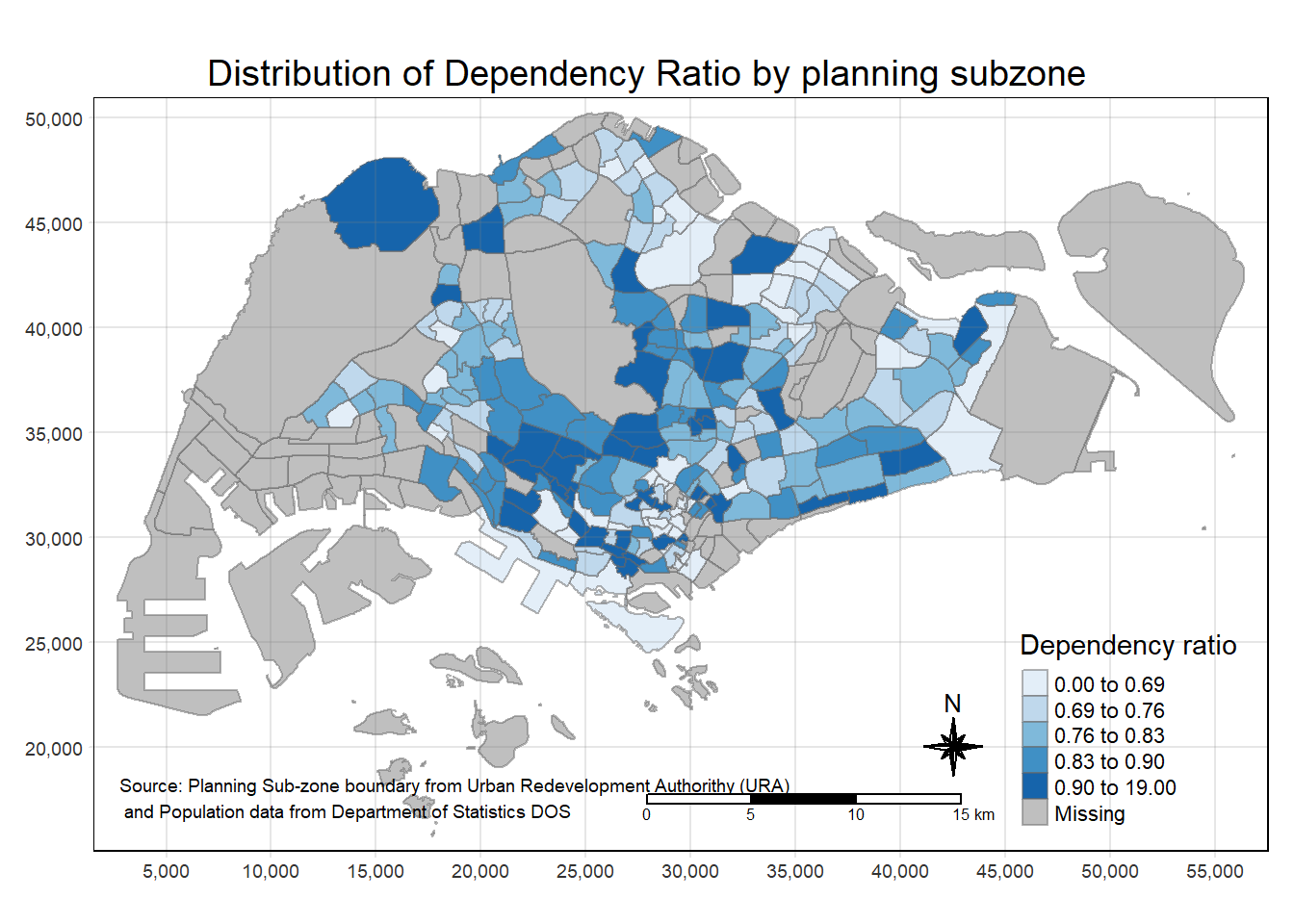
Anatomy of tmap
Base: tm_shape()
Layers: tm_fill(), tm_polygons()
tm_shape(mpsz_pop2020) +
  tm_polygons()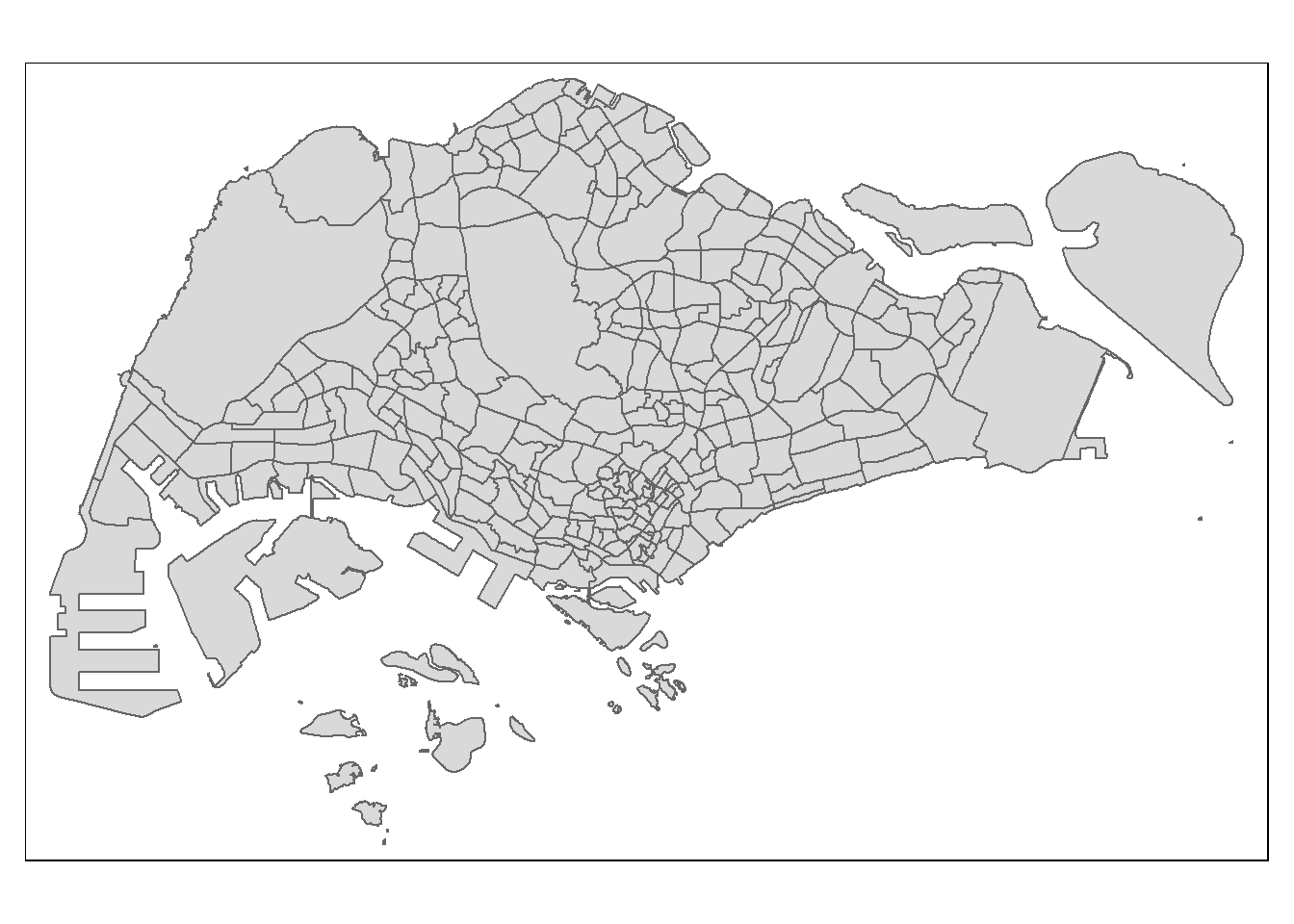
Using tm_polygons()
tm_shape(mpsz_pop2020)+
  tm_polygons("DEPENDENCY")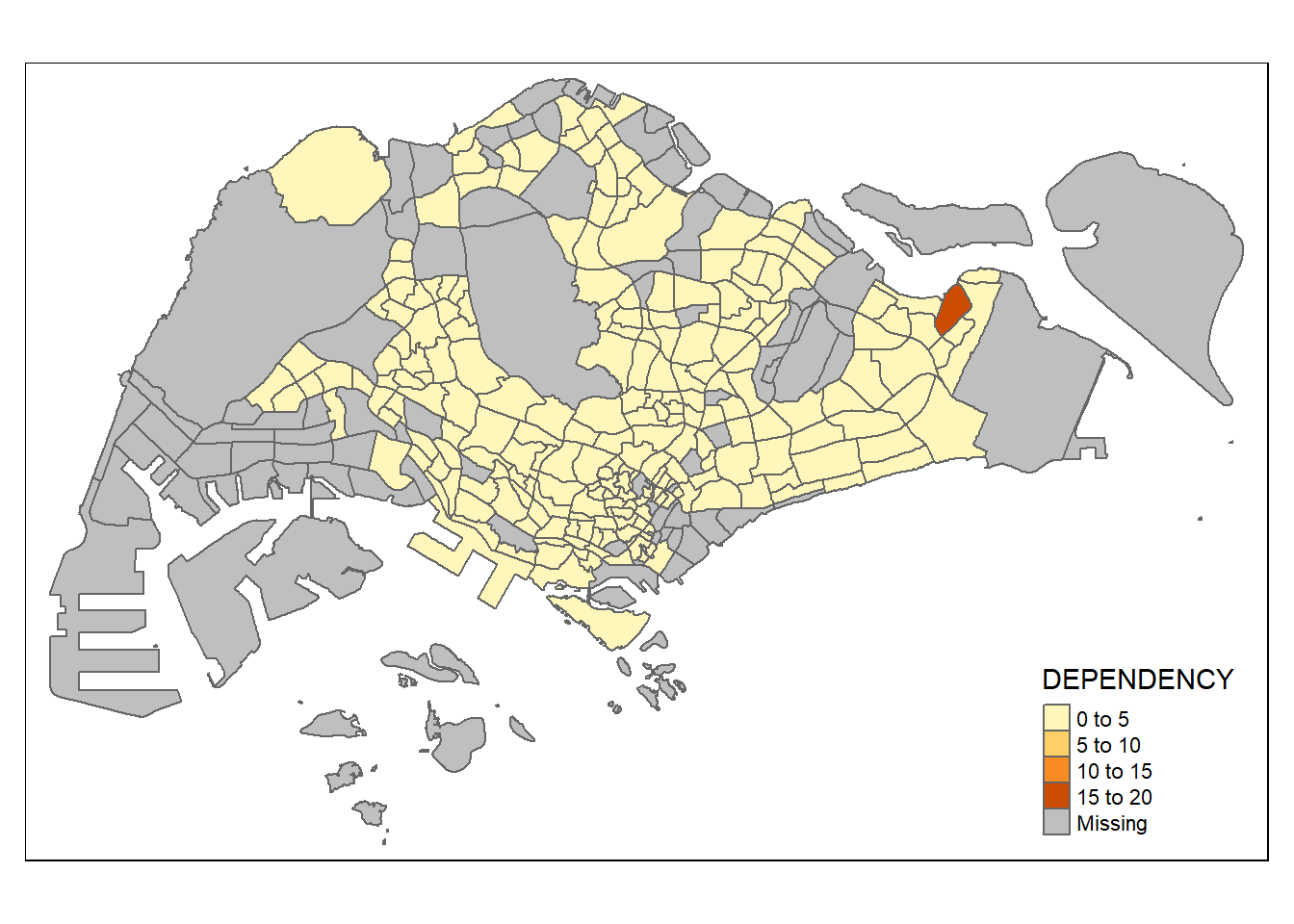
Using tm_fill()
tm_shape(mpsz_pop2020)+
  tm_fill("DEPENDENCY")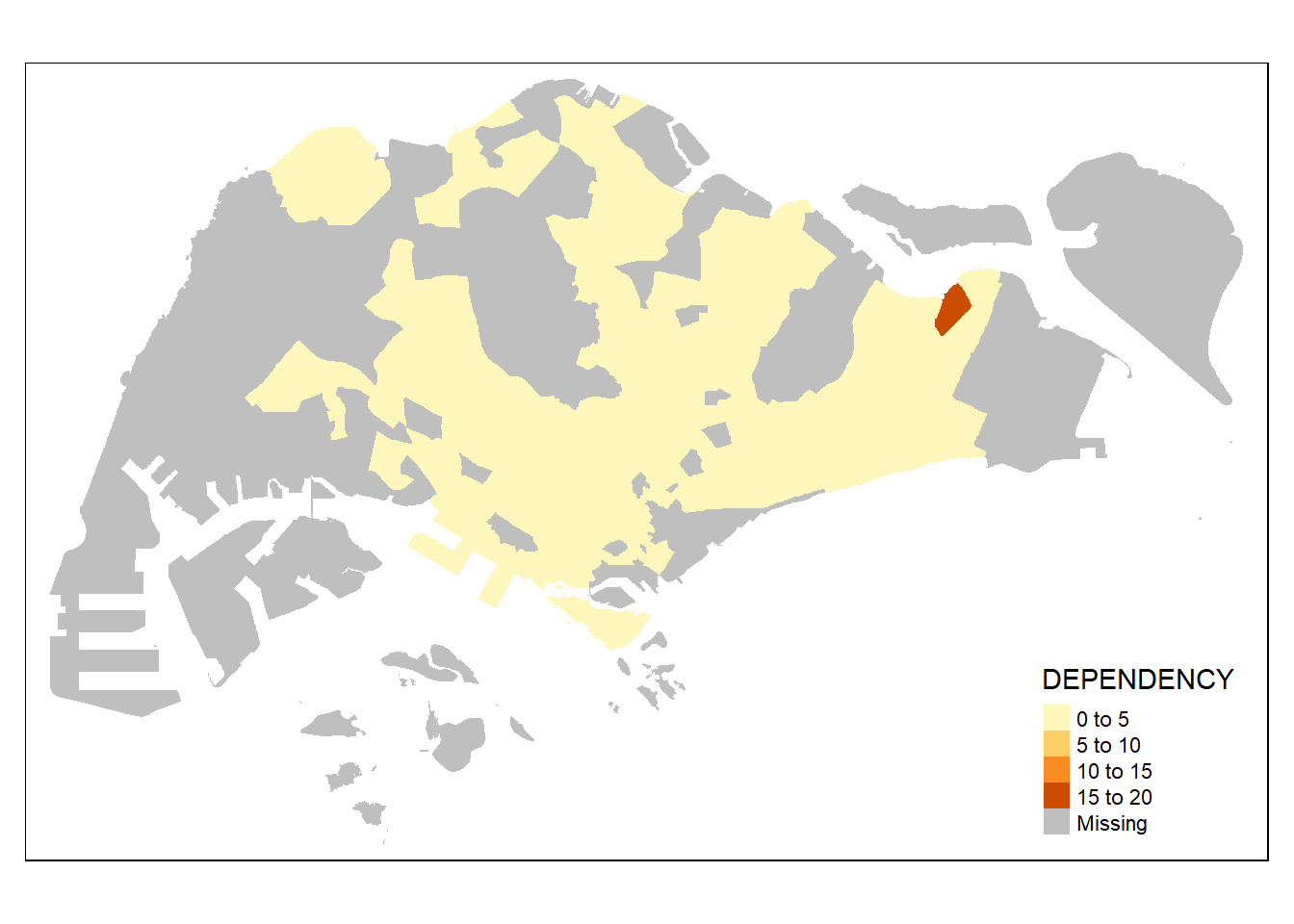
Give borders
tm_shape(mpsz_pop2020)+
  tm_fill("DEPENDENCY") +
  tm_borders(lwd = 0.1,  alpha = 1)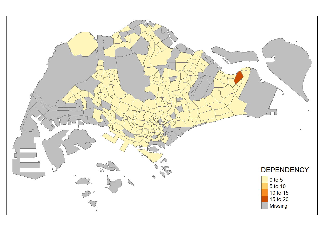
Data classification methods
Quantile data classification with 5 classes (built-in)
tm_shape(mpsz_pop2020)+
  tm_fill("DEPENDENCY",
          n = 5,
          style = "jenks") +
  tm_borders(alpha = 0.5)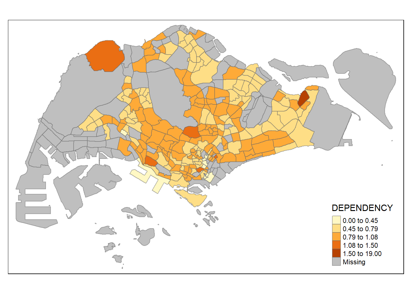
Custom category breaks
Check the summary statistics
summary(mpsz_pop2020$DEPENDENCY) Min. 1st Qu. Median Mean 3rd Qu. Max. NA's
0.0000 0.7113 0.7926 0.8561 0.8786 19.0000 92 We set break point at 0.60, 0.70, 0.80, 0.90. Additionally, we set minimum to 0 and maximum to 100.
tm_shape(mpsz_pop2020)+
  tm_fill("DEPENDENCY",
          breaks = c(0, 0.60, 0.70, 0.80, 0.90, 1.00)) +
  tm_borders(alpha = 0.5)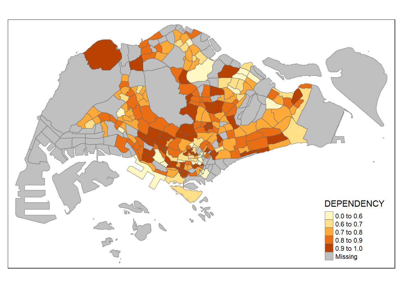
Color Scheme
Using ColourBrewer palette
tm_shape(mpsz_pop2020)+
  tm_fill("DEPENDENCY",
          n = 6,
          style = "quantile",
          palette = "Blues") +
  tm_borders(alpha = 0.5)
tm_shape(mpsz_pop2020)+
  tm_fill("DEPENDENCY",
          n = 6,
          style = "quantile",
          palette = "Blues") +
  tm_borders(alpha = 0.5)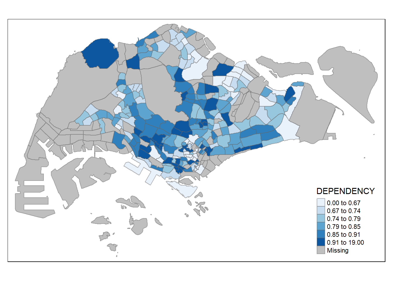
Map Layout
Whole cohesive map - title, scale bar, compass, margins, aspect ratios, legends, etc.
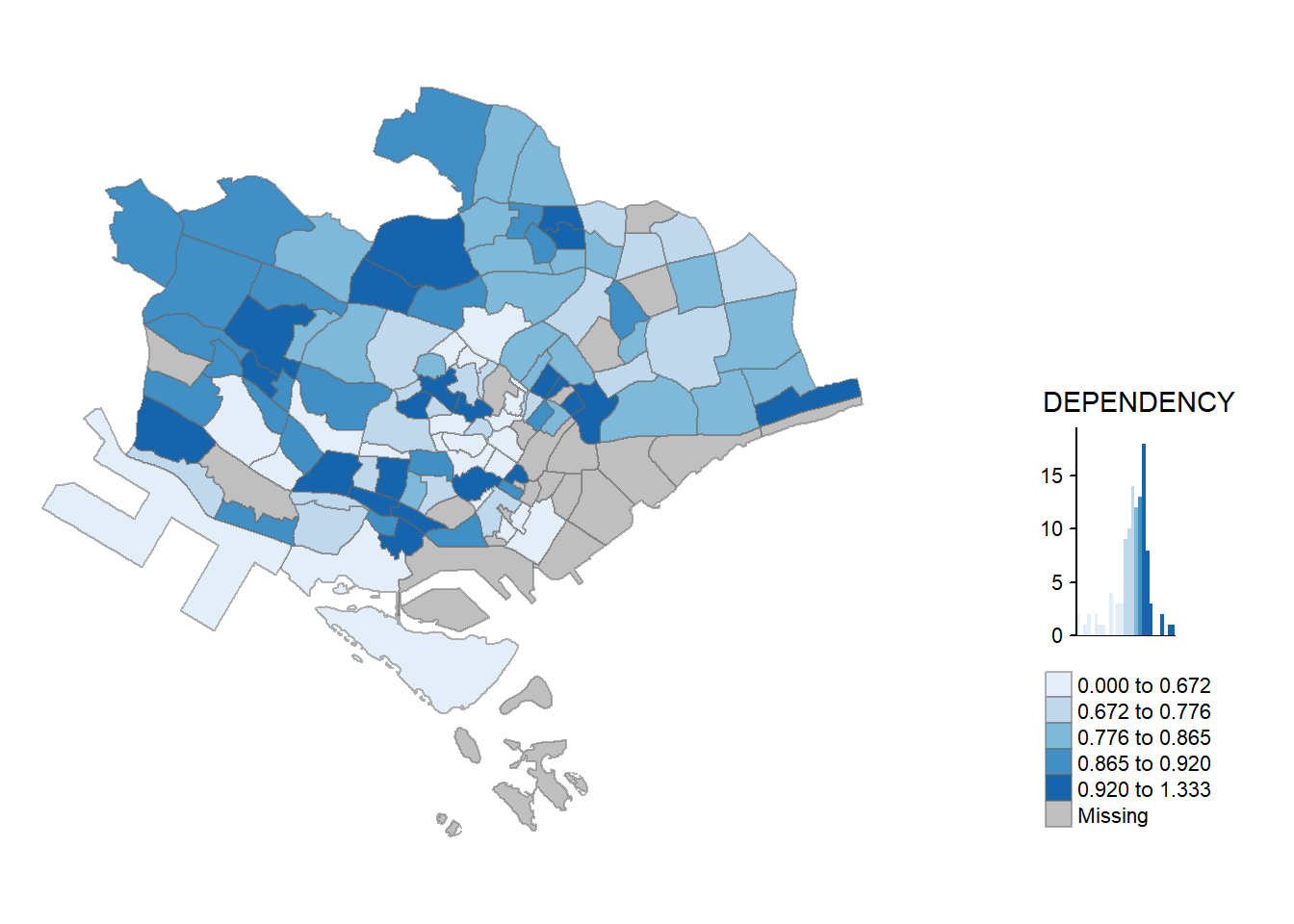
tm_shape(mpsz_pop2020)+
  tm_fill("DEPENDENCY",
          style = "jenks",
          palette = "Blues",
          legend.hist = TRUE,
          legend.is.portrait = TRUE,
          legend.hist.z = 0.1) +
  tm_layout(main.title = "Distribution of Dependency Ratio by planning subzone \n(Jenks classification)",
            main.title.position = "center",
            main.title.size = 1,
            legend.height = 0.45,
            legend.width = 0.35,
            legend.outside = FALSE,
            legend.position = c("right", "bottom"),
            frame = FALSE) +
  tm_borders(alpha = 0.5)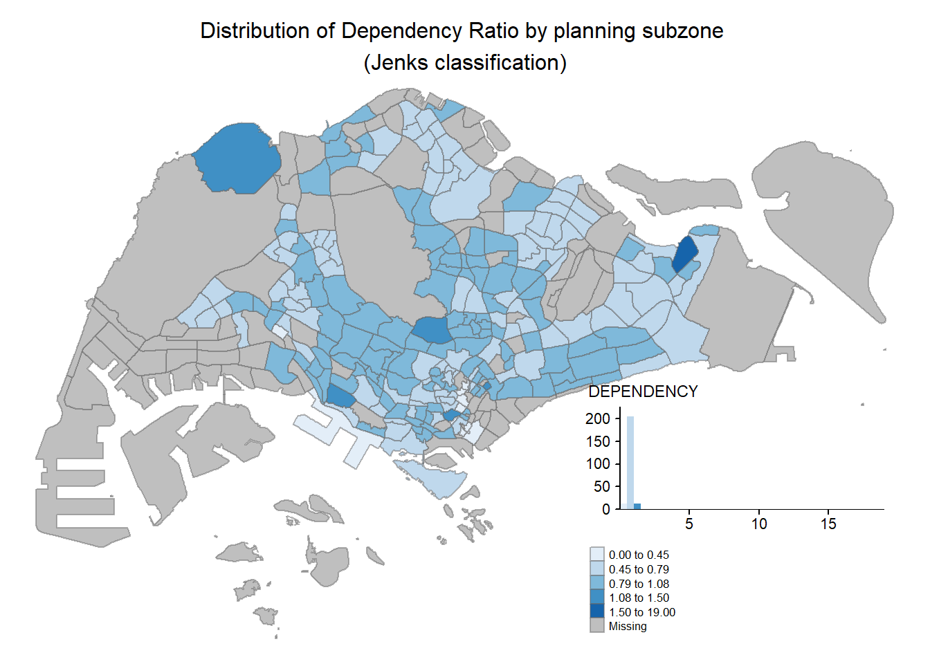
Map style
tm_shape(mpsz_pop2020)+
  tm_fill("DEPENDENCY",
          style = "quantile",
          palette = "-Greens") +
  tm_borders(alpha = 0.5) +
  tmap_style("classic")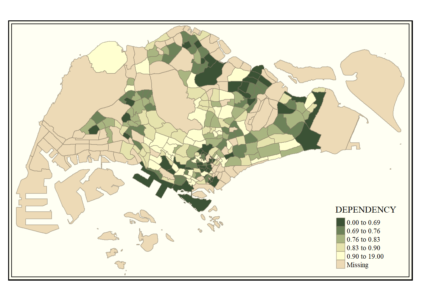
Cartographic furniture
tm_shape(mpsz_pop2020)+
  tm_fill("DEPENDENCY",
          style = "quantile",
          palette = "Blues",
          title = "No. of persons") +
  tm_layout(main.title = "Distribution of Dependency Ratio \nby planning subzone",
            main.title.position = "center",
            main.title.size = 1.2,
            legend.height = 0.45,
            legend.width = 0.35,
            frame = TRUE) +
  tm_borders(alpha = 0.5) +
  tm_compass(type="8star", size = 2) +
  tm_scale_bar(width = 0.15) +
  tm_grid(lwd = 0.1, alpha = 0.2) +
  tm_credits("Source: Planning Sub-zone boundary from Urban Redevelopment Authorithy (URA)\n and Population data from Department of Statistics DOS",
             position = c("left", "bottom"))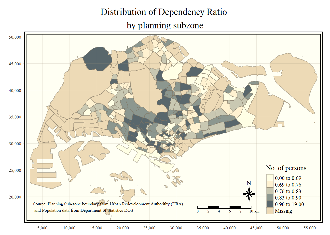
Small Multiples / Facets
Reset to default style
tmap_style("white")1. Assign multiple values to one of the aesthetic arguments
tm_shape(mpsz_pop2020)+
  tm_fill(c("YOUNG", "AGED"),
          style = "equal",
          palette = "Blues") +
  tm_layout(legend.position = c("right", "bottom")) +
  tm_borders(alpha = 0.5) +
  tmap_style("white")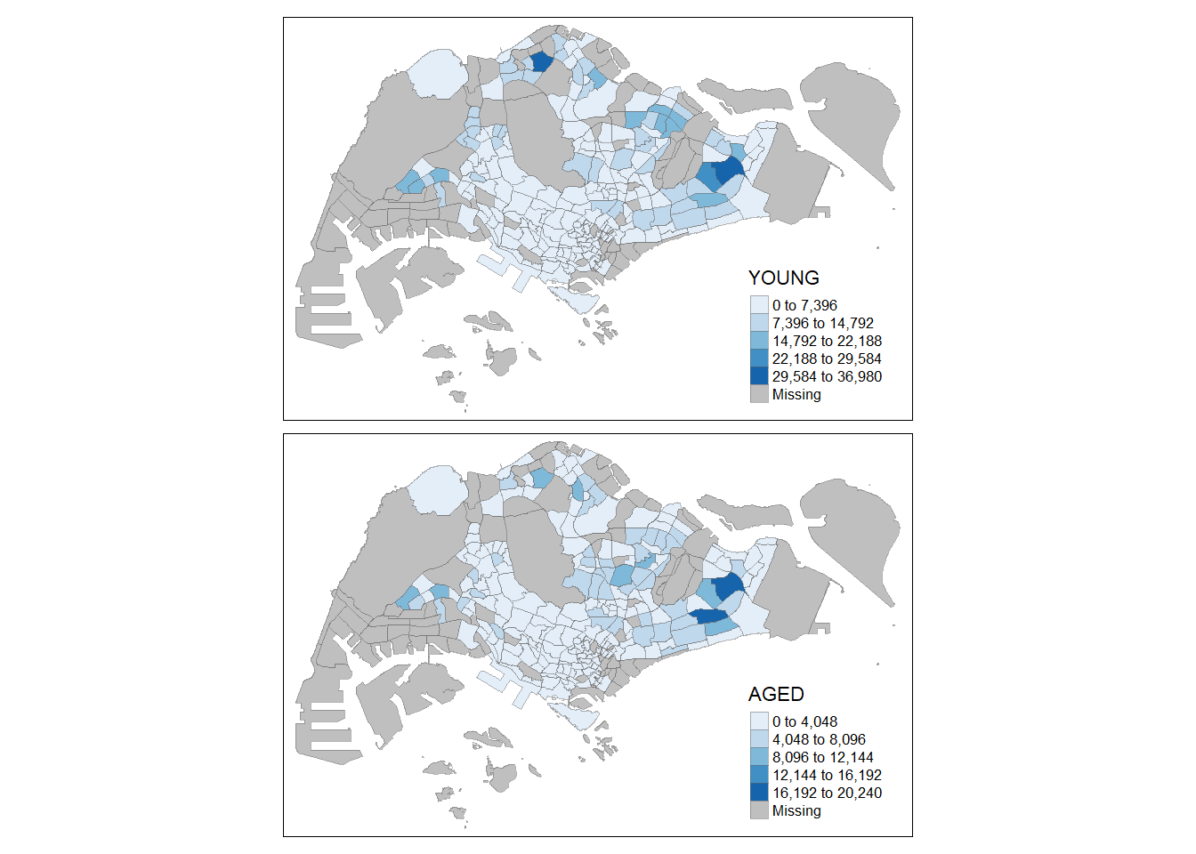
tm_shape(mpsz_pop2020)+
  tm_polygons(c("DEPENDENCY","AGED"),
          style = c("equal", "quantile"),
          palette = list("Blues","Greens")) +
  tm_layout(legend.position = c("right", "bottom"))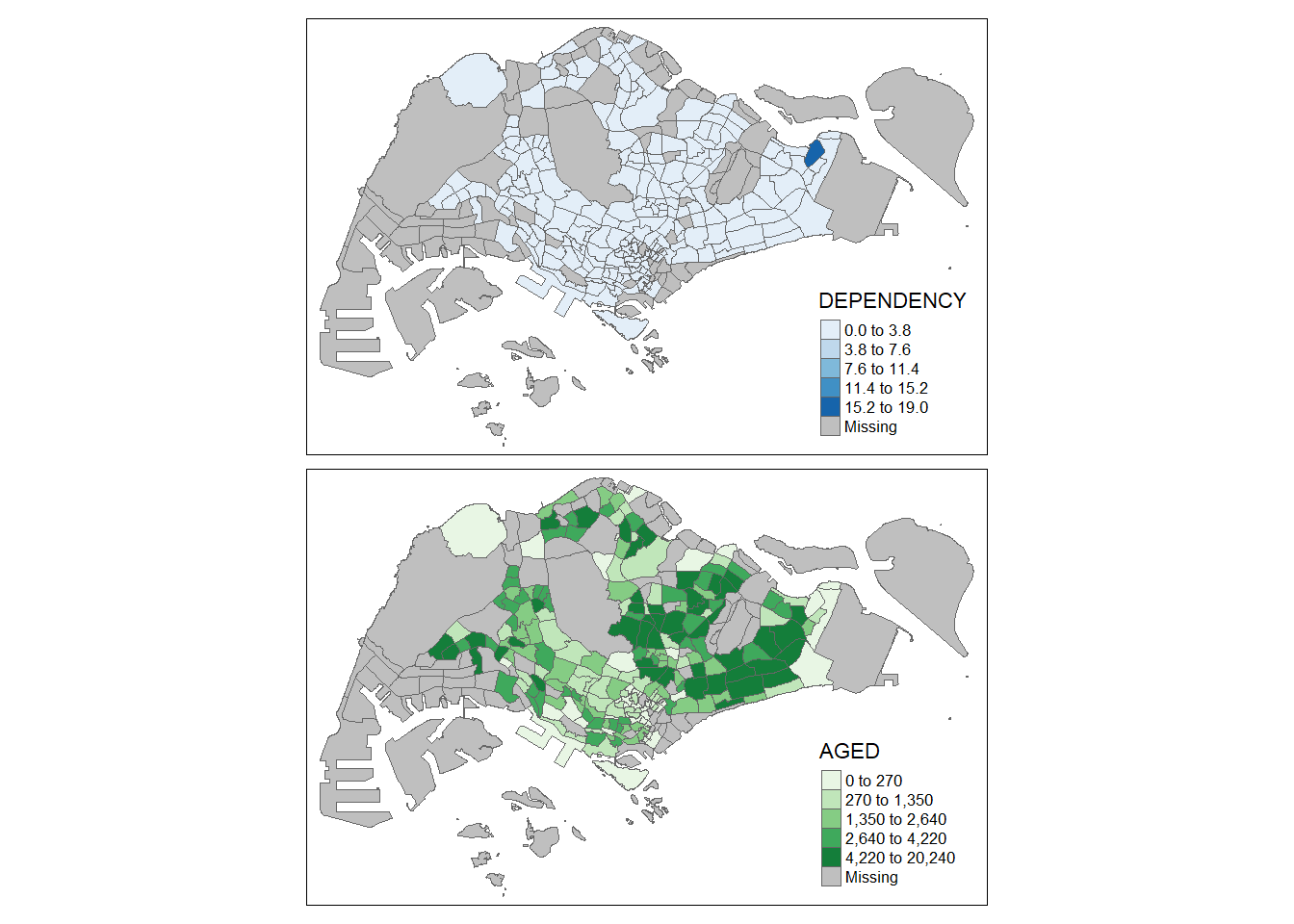
2. Define group-by variable in tm_facets()
tm_shape(mpsz_pop2020) +
  tm_fill("DEPENDENCY",
          style = "quantile",
          palette = "Blues",
          thres.poly = 0) +
  tm_facets(by="REGION_N",
            free.coords=TRUE,
            drop.shapes=TRUE) +
  tm_layout(legend.show = FALSE,
            title.position = c("center", "center"),
            title.size = 20) +
  tm_borders(alpha = 0.5)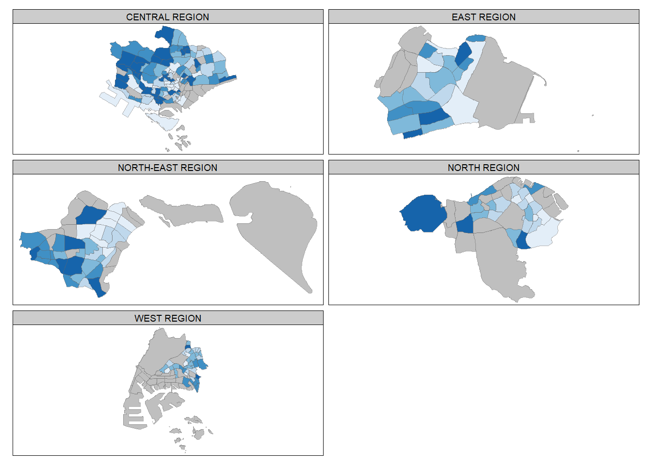
3. Multiple stand-alone maps with tmap_arrange()
youngmap <- tm_shape(mpsz_pop2020)+
  tm_polygons("YOUNG",
              style = "quantile",
              palette = "Blues")

agedmap <- tm_shape(mpsz_pop2020)+
  tm_polygons("AGED",
              style = "quantile",
              palette = "Blues")

tmap_arrange(youngmap, agedmap, asp=1, ncol=2)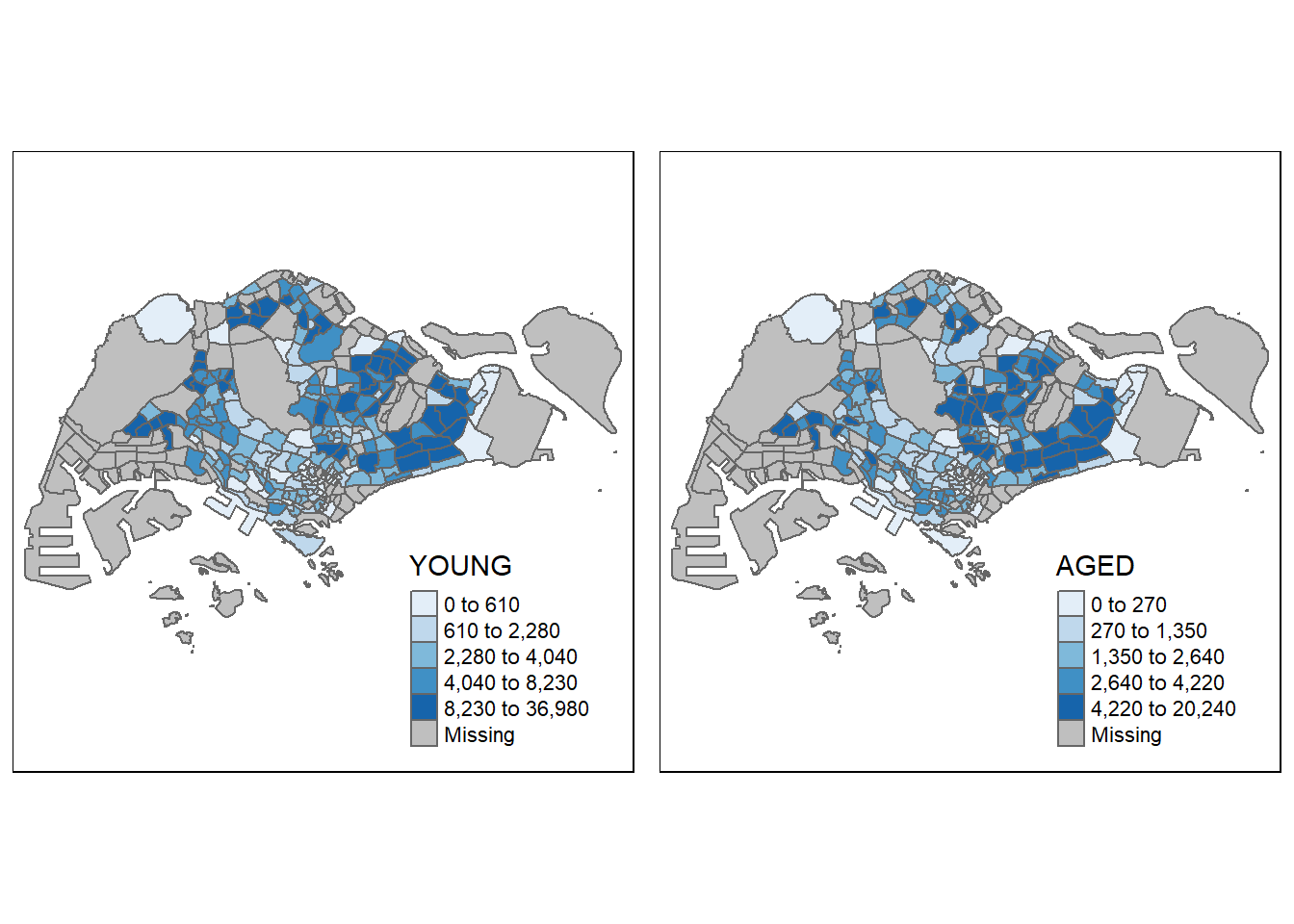
Mapping Spatial Object Meeting a Selection Criterion
tm_shape(mpsz_pop2020[mpsz_pop2020$REGION_N=="CENTRAL REGION", ])+
  tm_fill("DEPENDENCY",
          style = "quantile",
          palette = "Blues",
          legend.hist = TRUE,
          legend.is.portrait = TRUE,
          legend.hist.z = 0.1) +
  tm_layout(legend.outside = TRUE,
            legend.height = 0.45,
            legend.width = 5.0,
            legend.position = c("right", "bottom"),
            frame = FALSE) +
  tm_borders(alpha = 0.5)