pacman::p_load(maptools, sf, raster, spatstat, tmap)Hands-On Exercise 4 & 5: Spatial Point Patterns Analysis
Import packages
Importing Dataset
Spatial Data
childcare_sf <- st_read("data/geospatial/childcare.geojson") %>%
st_transform(crs = 3414)Reading layer `childcare' from data source
`C:\Jenpoer\IS415-GAA\Hands-On-Exercises\chapter-04\data\geospatial\childcare.geojson'
using driver `GeoJSON'
Simple feature collection with 1545 features and 2 fields
Geometry type: POINT
Dimension: XYZ
Bounding box: xmin: 103.6824 ymin: 1.248403 xmax: 103.9897 ymax: 1.462134
z_range: zmin: 0 zmax: 0
Geodetic CRS: WGS 84sg_sf <- st_read(dsn = "data/geospatial/CostalOutline", layer="CostalOutline")Reading layer `CostalOutline' from data source
`C:\Jenpoer\IS415-GAA\Hands-On-Exercises\chapter-04\data\geospatial\CostalOutline'
using driver `ESRI Shapefile'
Simple feature collection with 60 features and 4 fields
Geometry type: POLYGON
Dimension: XY
Bounding box: xmin: 2663.926 ymin: 16357.98 xmax: 56047.79 ymax: 50244.03
Projected CRS: SVY21mpsz_sf <- st_read(dsn = "../chapter-02/data/geospatial/master-plan-2014-subzone-boundary-web-shp",
layer = "MP14_SUBZONE_WEB_PL")Reading layer `MP14_SUBZONE_WEB_PL' from data source
`C:\Jenpoer\IS415-GAA\Hands-On-Exercises\chapter-02\data\geospatial\master-plan-2014-subzone-boundary-web-shp'
using driver `ESRI Shapefile'
Simple feature collection with 323 features and 15 fields
Geometry type: MULTIPOLYGON
Dimension: XY
Bounding box: xmin: 2667.538 ymin: 15748.72 xmax: 56396.44 ymax: 50256.33
Projected CRS: SVY21Retrieve referencing system information of geospatial data
Childcare: EPSG 3414, Projection CRS SVY21
st_geometry(childcare_sf)Geometry set for 1545 features
Geometry type: POINT
Dimension: XYZ
Bounding box: xmin: 11203.01 ymin: 25667.6 xmax: 45404.24 ymax: 49300.88
z_range: zmin: 0 zmax: 0
Projected CRS: SVY21 / Singapore TM
First 5 geometries:st_crs(childcare_sf)Coordinate Reference System:
User input: EPSG:3414
wkt:
PROJCRS["SVY21 / Singapore TM",
BASEGEOGCRS["SVY21",
DATUM["SVY21",
ELLIPSOID["WGS 84",6378137,298.257223563,
LENGTHUNIT["metre",1]]],
PRIMEM["Greenwich",0,
ANGLEUNIT["degree",0.0174532925199433]],
ID["EPSG",4757]],
CONVERSION["Singapore Transverse Mercator",
METHOD["Transverse Mercator",
ID["EPSG",9807]],
PARAMETER["Latitude of natural origin",1.36666666666667,
ANGLEUNIT["degree",0.0174532925199433],
ID["EPSG",8801]],
PARAMETER["Longitude of natural origin",103.833333333333,
ANGLEUNIT["degree",0.0174532925199433],
ID["EPSG",8802]],
PARAMETER["Scale factor at natural origin",1,
SCALEUNIT["unity",1],
ID["EPSG",8805]],
PARAMETER["False easting",28001.642,
LENGTHUNIT["metre",1],
ID["EPSG",8806]],
PARAMETER["False northing",38744.572,
LENGTHUNIT["metre",1],
ID["EPSG",8807]]],
CS[Cartesian,2],
AXIS["northing (N)",north,
ORDER[1],
LENGTHUNIT["metre",1]],
AXIS["easting (E)",east,
ORDER[2],
LENGTHUNIT["metre",1]],
USAGE[
SCOPE["Cadastre, engineering survey, topographic mapping."],
AREA["Singapore - onshore and offshore."],
BBOX[1.13,103.59,1.47,104.07]],
ID["EPSG",3414]]SG: EPSG 9001, Projection CRS SVY21
st_geometry(sg_sf)Geometry set for 60 features
Geometry type: POLYGON
Dimension: XY
Bounding box: xmin: 2663.926 ymin: 16357.98 xmax: 56047.79 ymax: 50244.03
Projected CRS: SVY21
First 5 geometries:st_crs(sg_sf)Coordinate Reference System:
User input: SVY21
wkt:
PROJCRS["SVY21",
BASEGEOGCRS["SVY21[WGS84]",
DATUM["World Geodetic System 1984",
ELLIPSOID["WGS 84",6378137,298.257223563,
LENGTHUNIT["metre",1]],
ID["EPSG",6326]],
PRIMEM["Greenwich",0,
ANGLEUNIT["Degree",0.0174532925199433]]],
CONVERSION["unnamed",
METHOD["Transverse Mercator",
ID["EPSG",9807]],
PARAMETER["Latitude of natural origin",1.36666666666667,
ANGLEUNIT["Degree",0.0174532925199433],
ID["EPSG",8801]],
PARAMETER["Longitude of natural origin",103.833333333333,
ANGLEUNIT["Degree",0.0174532925199433],
ID["EPSG",8802]],
PARAMETER["Scale factor at natural origin",1,
SCALEUNIT["unity",1],
ID["EPSG",8805]],
PARAMETER["False easting",28001.642,
LENGTHUNIT["metre",1],
ID["EPSG",8806]],
PARAMETER["False northing",38744.572,
LENGTHUNIT["metre",1],
ID["EPSG",8807]]],
CS[Cartesian,2],
AXIS["(E)",east,
ORDER[1],
LENGTHUNIT["metre",1,
ID["EPSG",9001]]],
AXIS["(N)",north,
ORDER[2],
LENGTHUNIT["metre",1,
ID["EPSG",9001]]]]MPSZ: EPSG 9001, Projection CRS SVY21
st_geometry(mpsz_sf)Geometry set for 323 features
Geometry type: MULTIPOLYGON
Dimension: XY
Bounding box: xmin: 2667.538 ymin: 15748.72 xmax: 56396.44 ymax: 50256.33
Projected CRS: SVY21
First 5 geometries:st_crs(mpsz_sf)Coordinate Reference System:
User input: SVY21
wkt:
PROJCRS["SVY21",
BASEGEOGCRS["SVY21[WGS84]",
DATUM["World Geodetic System 1984",
ELLIPSOID["WGS 84",6378137,298.257223563,
LENGTHUNIT["metre",1]],
ID["EPSG",6326]],
PRIMEM["Greenwich",0,
ANGLEUNIT["Degree",0.0174532925199433]]],
CONVERSION["unnamed",
METHOD["Transverse Mercator",
ID["EPSG",9807]],
PARAMETER["Latitude of natural origin",1.36666666666667,
ANGLEUNIT["Degree",0.0174532925199433],
ID["EPSG",8801]],
PARAMETER["Longitude of natural origin",103.833333333333,
ANGLEUNIT["Degree",0.0174532925199433],
ID["EPSG",8802]],
PARAMETER["Scale factor at natural origin",1,
SCALEUNIT["unity",1],
ID["EPSG",8805]],
PARAMETER["False easting",28001.642,
LENGTHUNIT["metre",1],
ID["EPSG",8806]],
PARAMETER["False northing",38744.572,
LENGTHUNIT["metre",1],
ID["EPSG",8807]]],
CS[Cartesian,2],
AXIS["(E)",east,
ORDER[1],
LENGTHUNIT["metre",1,
ID["EPSG",9001]]],
AXIS["(N)",north,
ORDER[2],
LENGTHUNIT["metre",1,
ID["EPSG",9001]]]]Assign correct crs information
SG & MPSZ
We only need to change the crs because it is already the correct projection.
mpsz_sf <- st_set_crs(mpsz_sf, 3414)
sg_sf <- st_set_crs(sg_sf, 3414)Mapping
tmap_mode("plot")
tm_shape(mpsz_sf) +
tm_polygons() +
tm_shape(childcare_sf) +
tm_dots()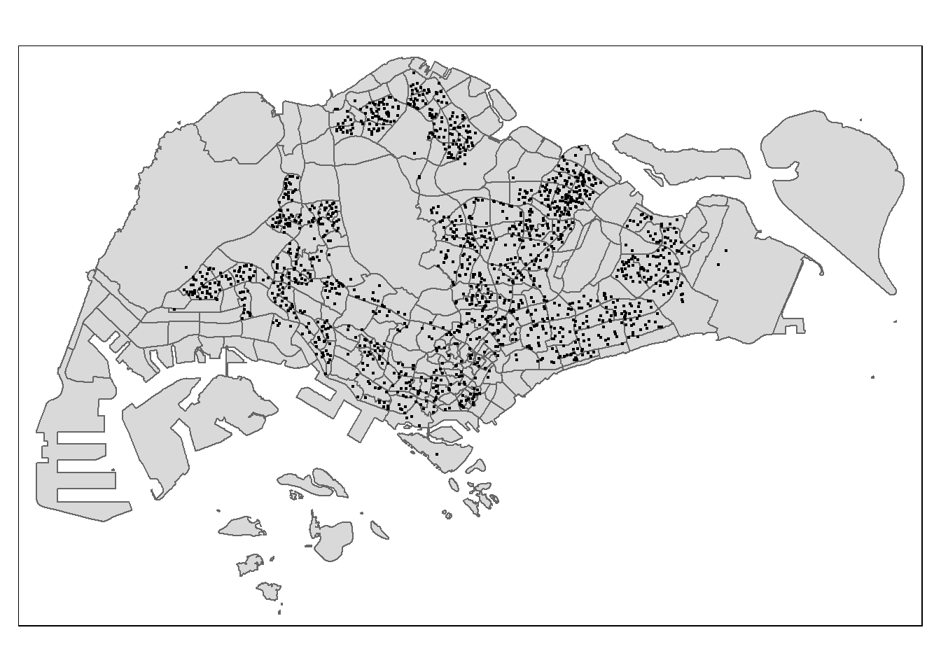
tmap_mode('view')
tm_shape(childcare_sf)+
tm_dots()tmap_mode("plot")Geospatial Data Wrangling
Conversion from sf’s simple feature data frame to sp’s Spatial* class
childcare <- as_Spatial(childcare_sf)
mpsz <- as_Spatial(mpsz_sf)
sg <- as_Spatial(sg_sf)summary(childcare)Object of class SpatialPointsDataFrame
Coordinates:
min max
coords.x1 11203.01 45404.24
coords.x2 25667.60 49300.88
coords.x3 0.00 0.00
Is projected: TRUE
proj4string :
[+proj=tmerc +lat_0=1.36666666666667 +lon_0=103.833333333333 +k=1
+x_0=28001.642 +y_0=38744.572 +ellps=WGS84 +towgs84=0,0,0,0,0,0,0
+units=m +no_defs]
Number of points: 1545
Data attributes:
Name Description
Length:1545 Length:1545
Class :character Class :character
Mode :character Mode :character summary(mpsz)Object of class SpatialPolygonsDataFrame
Coordinates:
min max
x 2667.538 56396.44
y 15748.721 50256.33
Is projected: TRUE
proj4string :
[+proj=tmerc +lat_0=1.36666666666667 +lon_0=103.833333333333 +k=1
+x_0=28001.642 +y_0=38744.572 +ellps=WGS84 +towgs84=0,0,0,0,0,0,0
+units=m +no_defs]
Data attributes:
OBJECTID SUBZONE_NO SUBZONE_N SUBZONE_C
Min. : 1.0 Min. : 1.000 Length:323 Length:323
1st Qu.: 81.5 1st Qu.: 2.000 Class :character Class :character
Median :162.0 Median : 4.000 Mode :character Mode :character
Mean :162.0 Mean : 4.625
3rd Qu.:242.5 3rd Qu.: 6.500
Max. :323.0 Max. :17.000
CA_IND PLN_AREA_N PLN_AREA_C REGION_N
Length:323 Length:323 Length:323 Length:323
Class :character Class :character Class :character Class :character
Mode :character Mode :character Mode :character Mode :character
REGION_C INC_CRC FMEL_UPD_D X_ADDR
Length:323 Length:323 Min. :2014-12-05 Min. : 5093
Class :character Class :character 1st Qu.:2014-12-05 1st Qu.:21864
Mode :character Mode :character Median :2014-12-05 Median :28465
Mean :2014-12-05 Mean :27257
3rd Qu.:2014-12-05 3rd Qu.:31674
Max. :2014-12-05 Max. :50425
Y_ADDR SHAPE_Leng SHAPE_Area
Min. :19579 Min. : 871.5 Min. : 39438
1st Qu.:31776 1st Qu.: 3709.6 1st Qu.: 628261
Median :35113 Median : 5211.9 Median : 1229894
Mean :36106 Mean : 6524.4 Mean : 2420882
3rd Qu.:39869 3rd Qu.: 6942.6 3rd Qu.: 2106483
Max. :49553 Max. :68083.9 Max. :69748299 summary(sg)Object of class SpatialPolygonsDataFrame
Coordinates:
min max
x 2663.926 56047.79
y 16357.981 50244.03
Is projected: TRUE
proj4string :
[+proj=tmerc +lat_0=1.36666666666667 +lon_0=103.833333333333 +k=1
+x_0=28001.642 +y_0=38744.572 +ellps=WGS84 +towgs84=0,0,0,0,0,0,0
+units=m +no_defs]
Data attributes:
GDO_GID MSLINK MAPID COSTAL_NAM
Min. : 1.00 Min. : 1.00 Min. :0 Length:60
1st Qu.:15.75 1st Qu.:17.75 1st Qu.:0 Class :character
Median :30.50 Median :33.50 Median :0 Mode :character
Mean :30.50 Mean :33.77 Mean :0
3rd Qu.:45.25 3rd Qu.:49.25 3rd Qu.:0
Max. :60.00 Max. :67.00 Max. :0 Conversion from Spatial* class to generic sp format (Spatial)
childcare_sp <- as(childcare, "SpatialPoints")
sg_sp <- as(sg, "SpatialPolygons")childcare_spclass : SpatialPoints
features : 1545
extent : 11203.01, 45404.24, 25667.6, 49300.88 (xmin, xmax, ymin, ymax)
crs : +proj=tmerc +lat_0=1.36666666666667 +lon_0=103.833333333333 +k=1 +x_0=28001.642 +y_0=38744.572 +ellps=WGS84 +towgs84=0,0,0,0,0,0,0 +units=m +no_defs sg_spclass : SpatialPolygons
features : 60
extent : 2663.926, 56047.79, 16357.98, 50244.03 (xmin, xmax, ymin, ymax)
crs : +proj=tmerc +lat_0=1.36666666666667 +lon_0=103.833333333333 +k=1 +x_0=28001.642 +y_0=38744.572 +ellps=WGS84 +towgs84=0,0,0,0,0,0,0 +units=m +no_defs Conversion from generic sp format to spatstat’s ppp
childcare_ppp <- as(childcare_sp, "ppp")
childcare_pppPlanar point pattern: 1545 points
window: rectangle = [11203.01, 45404.24] x [25667.6, 49300.88] unitsplot(childcare_ppp)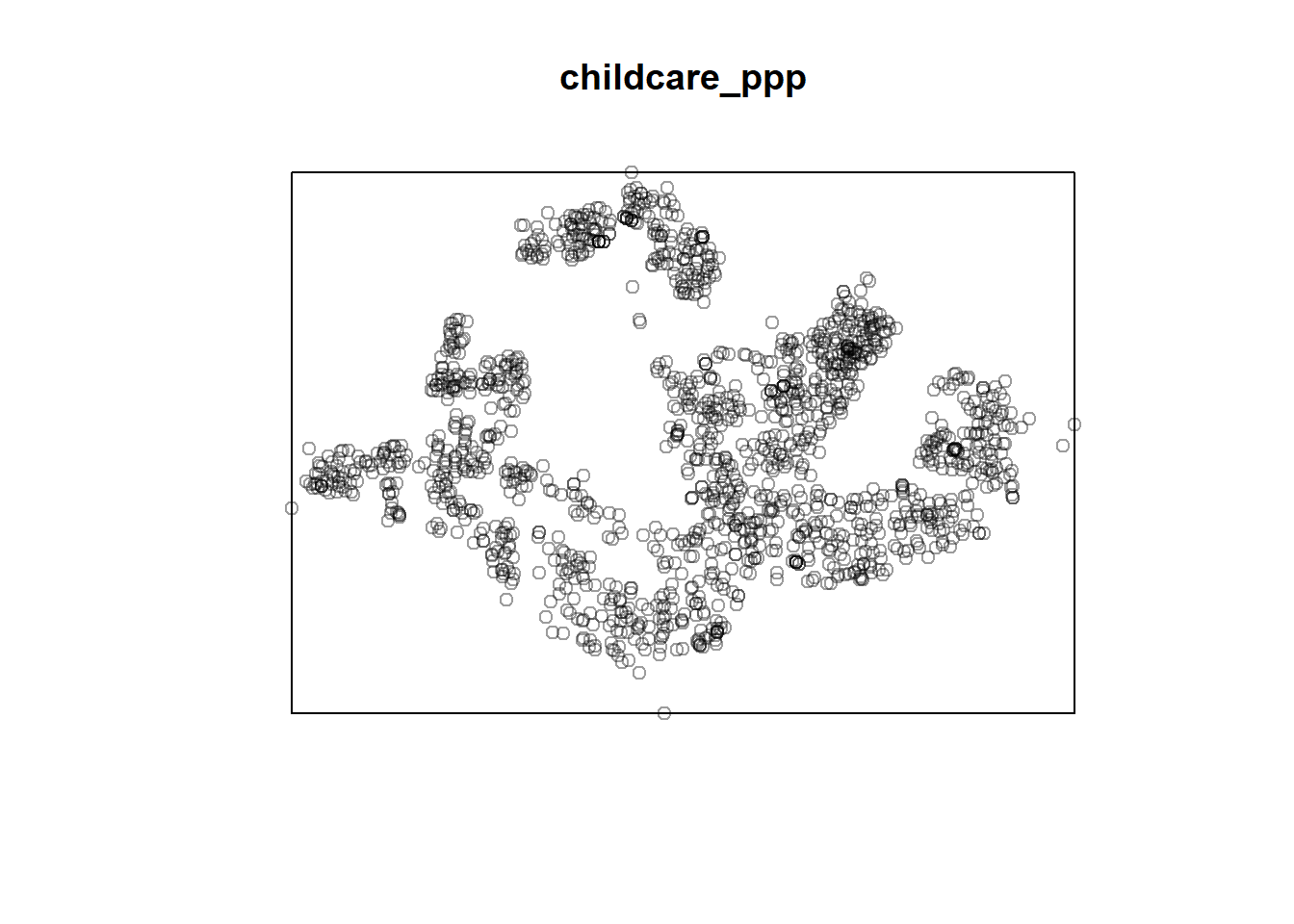
summary(childcare_ppp)Planar point pattern: 1545 points
Average intensity 1.91145e-06 points per square unit
*Pattern contains duplicated points*
Coordinates are given to 3 decimal places
i.e. rounded to the nearest multiple of 0.001 units
Window: rectangle = [11203.01, 45404.24] x [25667.6, 49300.88] units
(34200 x 23630 units)
Window area = 808287000 square units
Duplicated points may be problematic in spatial point patterns analysis. This is because the statistical methodology used for spatial point patterns analysis assumes that points cannot be coincident.
Handling duplicated points
Check for duplication
any(duplicated(childcare_ppp))[1] TRUECount the number of coincident points
sum(multiplicity(childcare_ppp) > 1)[1] 128View locations of duplicate point events
tmap_mode('view')
tm_shape(childcare) +
tm_dots(alpha=0.4,
size=0.05)We can see duplicate points because they are more opaque (multiple points overlapping exactly on the same spot).
tmap_mode('plot')There are three approaches to this problem.
- Delete the duplicates: But some useful point events will be lost.
- Jittering: Add a small perturbation to the duplicate points so that they do not occupy the exact same space.
- Marks: make each point “unique” and then attach the duplicates of the points to the patterns as marks (attributes of the points). Then, we need analytical techniques that take into account these marks.
This code implements jittering.
childcare_ppp_jit <- rjitter(childcare_ppp,
retru=TRUE,
nsim=1,
drop=TRUE)any(duplicated(childcare_ppp_jit))[1] FALSECreating spatstat’s owin object
spatstat’s owin object is specially designed to represent a polygonal region.
sg_owin <- as(sg_sp, "owin")plot(sg_owin)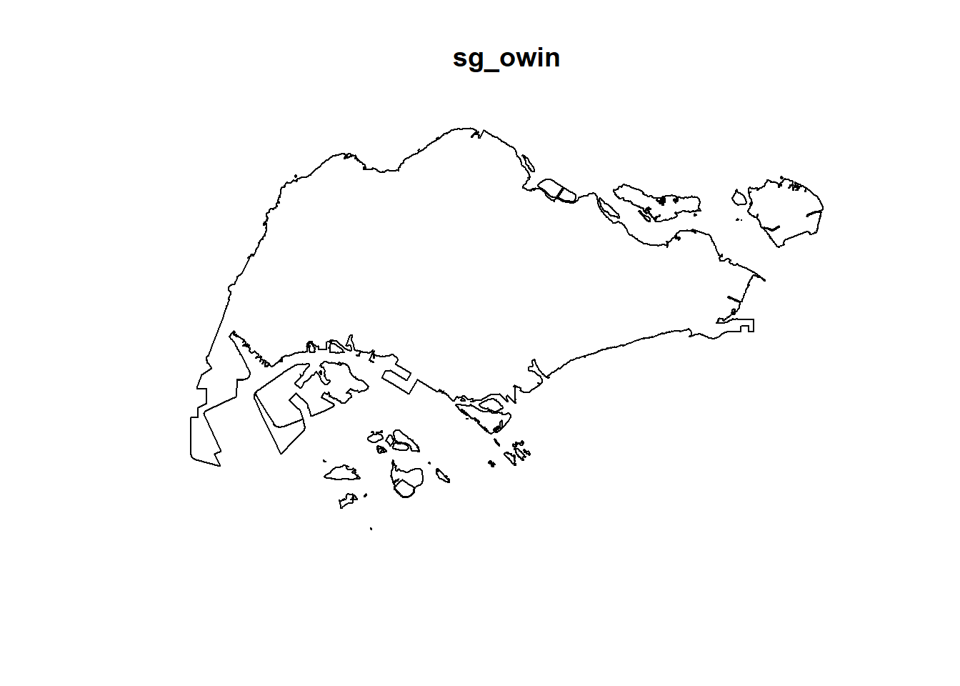
summary(sg_owin)Window: polygonal boundary
60 separate polygons (no holes)
vertices area relative.area
polygon 1 38 1.56140e+04 2.09e-05
polygon 2 735 4.69093e+06 6.27e-03
polygon 3 49 1.66986e+04 2.23e-05
polygon 4 76 3.12332e+05 4.17e-04
polygon 5 5141 6.36179e+08 8.50e-01
polygon 6 42 5.58317e+04 7.46e-05
polygon 7 67 1.31354e+06 1.75e-03
polygon 8 15 4.46420e+03 5.96e-06
polygon 9 14 5.46674e+03 7.30e-06
polygon 10 37 5.26194e+03 7.03e-06
polygon 11 53 3.44003e+04 4.59e-05
polygon 12 74 5.82234e+04 7.78e-05
polygon 13 69 5.63134e+04 7.52e-05
polygon 14 143 1.45139e+05 1.94e-04
polygon 15 165 3.38736e+05 4.52e-04
polygon 16 130 9.40465e+04 1.26e-04
polygon 17 19 1.80977e+03 2.42e-06
polygon 18 16 2.01046e+03 2.69e-06
polygon 19 93 4.30642e+05 5.75e-04
polygon 20 90 4.15092e+05 5.54e-04
polygon 21 721 1.92795e+06 2.57e-03
polygon 22 330 1.11896e+06 1.49e-03
polygon 23 115 9.28394e+05 1.24e-03
polygon 24 37 1.01705e+04 1.36e-05
polygon 25 25 1.66227e+04 2.22e-05
polygon 26 10 2.14507e+03 2.86e-06
polygon 27 190 2.02489e+05 2.70e-04
polygon 28 175 9.25904e+05 1.24e-03
polygon 29 1993 9.99217e+06 1.33e-02
polygon 30 38 2.42492e+04 3.24e-05
polygon 31 24 6.35239e+03 8.48e-06
polygon 32 53 6.35791e+05 8.49e-04
polygon 33 41 1.60161e+04 2.14e-05
polygon 34 22 2.54368e+03 3.40e-06
polygon 35 30 1.08382e+04 1.45e-05
polygon 36 327 2.16921e+06 2.90e-03
polygon 37 111 6.62927e+05 8.85e-04
polygon 38 90 1.15991e+05 1.55e-04
polygon 39 98 6.26829e+04 8.37e-05
polygon 40 415 3.25384e+06 4.35e-03
polygon 41 222 1.51142e+06 2.02e-03
polygon 42 107 6.33039e+05 8.45e-04
polygon 43 7 2.48299e+03 3.32e-06
polygon 44 17 3.28303e+04 4.38e-05
polygon 45 26 8.34758e+03 1.11e-05
polygon 46 177 4.67446e+05 6.24e-04
polygon 47 16 3.19460e+03 4.27e-06
polygon 48 15 4.87296e+03 6.51e-06
polygon 49 66 1.61841e+04 2.16e-05
polygon 50 149 5.63430e+06 7.53e-03
polygon 51 609 2.62570e+07 3.51e-02
polygon 52 8 7.82256e+03 1.04e-05
polygon 53 976 2.33447e+07 3.12e-02
polygon 54 55 8.25379e+04 1.10e-04
polygon 55 976 2.33447e+07 3.12e-02
polygon 56 61 3.33449e+05 4.45e-04
polygon 57 6 1.68410e+04 2.25e-05
polygon 58 4 9.45963e+03 1.26e-05
polygon 59 46 6.99702e+05 9.35e-04
polygon 60 13 7.00873e+04 9.36e-05
enclosing rectangle: [2663.93, 56047.79] x [16357.98, 50244.03] units
(53380 x 33890 units)
Window area = 748741000 square units
Fraction of frame area: 0.414Combining point events object and owin object
childcareSG_ppp = childcare_ppp[sg_owin]summary(childcareSG_ppp)Planar point pattern: 1545 points
Average intensity 2.063463e-06 points per square unit
*Pattern contains duplicated points*
Coordinates are given to 3 decimal places
i.e. rounded to the nearest multiple of 0.001 units
Window: polygonal boundary
60 separate polygons (no holes)
vertices area relative.area
polygon 1 38 1.56140e+04 2.09e-05
polygon 2 735 4.69093e+06 6.27e-03
polygon 3 49 1.66986e+04 2.23e-05
polygon 4 76 3.12332e+05 4.17e-04
polygon 5 5141 6.36179e+08 8.50e-01
polygon 6 42 5.58317e+04 7.46e-05
polygon 7 67 1.31354e+06 1.75e-03
polygon 8 15 4.46420e+03 5.96e-06
polygon 9 14 5.46674e+03 7.30e-06
polygon 10 37 5.26194e+03 7.03e-06
polygon 11 53 3.44003e+04 4.59e-05
polygon 12 74 5.82234e+04 7.78e-05
polygon 13 69 5.63134e+04 7.52e-05
polygon 14 143 1.45139e+05 1.94e-04
polygon 15 165 3.38736e+05 4.52e-04
polygon 16 130 9.40465e+04 1.26e-04
polygon 17 19 1.80977e+03 2.42e-06
polygon 18 16 2.01046e+03 2.69e-06
polygon 19 93 4.30642e+05 5.75e-04
polygon 20 90 4.15092e+05 5.54e-04
polygon 21 721 1.92795e+06 2.57e-03
polygon 22 330 1.11896e+06 1.49e-03
polygon 23 115 9.28394e+05 1.24e-03
polygon 24 37 1.01705e+04 1.36e-05
polygon 25 25 1.66227e+04 2.22e-05
polygon 26 10 2.14507e+03 2.86e-06
polygon 27 190 2.02489e+05 2.70e-04
polygon 28 175 9.25904e+05 1.24e-03
polygon 29 1993 9.99217e+06 1.33e-02
polygon 30 38 2.42492e+04 3.24e-05
polygon 31 24 6.35239e+03 8.48e-06
polygon 32 53 6.35791e+05 8.49e-04
polygon 33 41 1.60161e+04 2.14e-05
polygon 34 22 2.54368e+03 3.40e-06
polygon 35 30 1.08382e+04 1.45e-05
polygon 36 327 2.16921e+06 2.90e-03
polygon 37 111 6.62927e+05 8.85e-04
polygon 38 90 1.15991e+05 1.55e-04
polygon 39 98 6.26829e+04 8.37e-05
polygon 40 415 3.25384e+06 4.35e-03
polygon 41 222 1.51142e+06 2.02e-03
polygon 42 107 6.33039e+05 8.45e-04
polygon 43 7 2.48299e+03 3.32e-06
polygon 44 17 3.28303e+04 4.38e-05
polygon 45 26 8.34758e+03 1.11e-05
polygon 46 177 4.67446e+05 6.24e-04
polygon 47 16 3.19460e+03 4.27e-06
polygon 48 15 4.87296e+03 6.51e-06
polygon 49 66 1.61841e+04 2.16e-05
polygon 50 149 5.63430e+06 7.53e-03
polygon 51 609 2.62570e+07 3.51e-02
polygon 52 8 7.82256e+03 1.04e-05
polygon 53 976 2.33447e+07 3.12e-02
polygon 54 55 8.25379e+04 1.10e-04
polygon 55 976 2.33447e+07 3.12e-02
polygon 56 61 3.33449e+05 4.45e-04
polygon 57 6 1.68410e+04 2.25e-05
polygon 58 4 9.45963e+03 1.26e-05
polygon 59 46 6.99702e+05 9.35e-04
polygon 60 13 7.00873e+04 9.36e-05
enclosing rectangle: [2663.93, 56047.79] x [16357.98, 50244.03] units
(53380 x 33890 units)
Window area = 748741000 square units
Fraction of frame area: 0.414plot(childcareSG_ppp)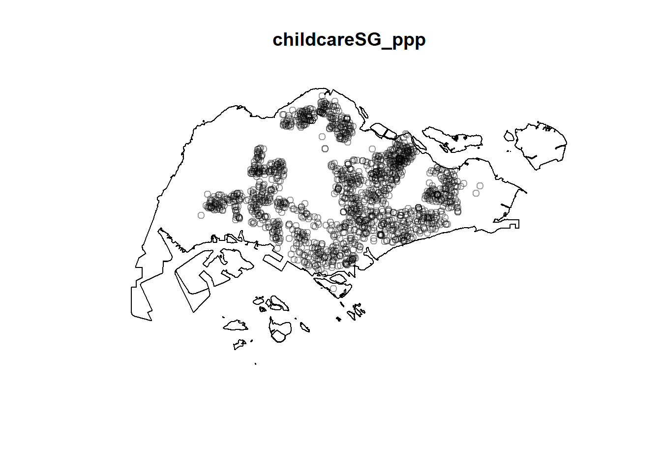
First-order Spatial Point Patterns Analysis (Hands-On Exercise 4)
Kernel Density Estimation
Computing KDE using automatic bandwidth selection method
kde_childcareSG_bw <- density(childcareSG_ppp,
sigma=bw.diggle,
edge=TRUE,
kernel="gaussian")plot(kde_childcareSG_bw)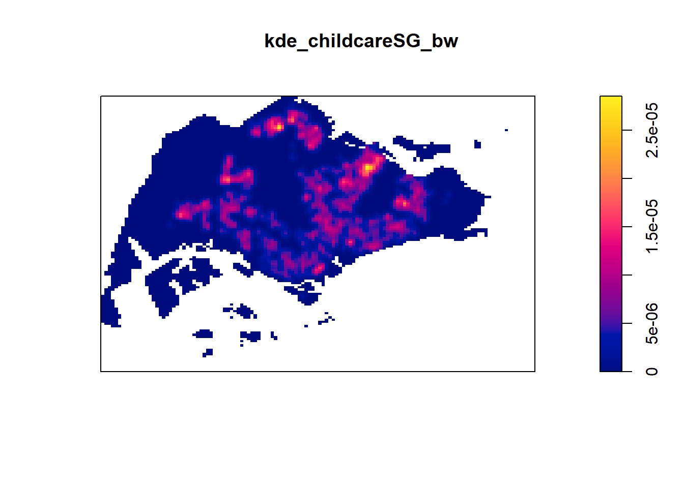
Bandwidth:
bw <- bw.diggle(childcareSG_ppp)
bw sigma
298.4095 Rescaling KDE values
childcareSG_ppp.km <- rescale(childcareSG_ppp, 1000, "km")kde_childcareSG.bw <- density(childcareSG_ppp.km, sigma=bw.diggle, edge=TRUE, kernel="gaussian")
plot(kde_childcareSG.bw)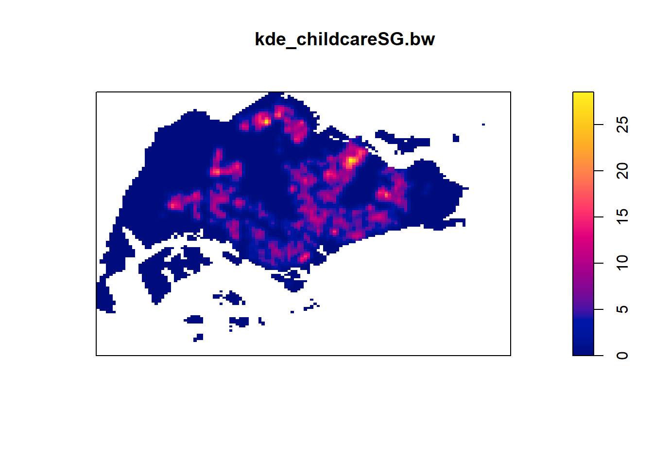
Different automatic bandwidth methods
bw.CvL(childcareSG_ppp.km) sigma
4.543278 bw.scott(childcareSG_ppp.km) sigma.x sigma.y
2.224898 1.450966 bw.ppl(childcareSG_ppp.km) sigma
0.3897114 bw.diggle(childcareSG_ppp.km) sigma
0.2984095 bw.diggle vs bw.ppl
kde_childcareSG.ppl <- density(childcareSG_ppp.km,
sigma=bw.ppl,
edge=TRUE,
kernel="gaussian")
par(mfrow=c(1,2))
plot(kde_childcareSG.bw, main = "bw.diggle")
plot(kde_childcareSG.ppl, main = "bw.ppl")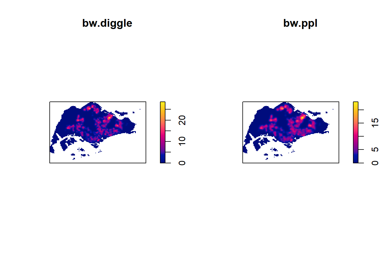
par(mfrow=c(2,2))
plot(density(childcareSG_ppp.km,
sigma=bw.ppl,
edge=TRUE,
kernel="gaussian"),
main="Gaussian")
plot(density(childcareSG_ppp.km,
sigma=bw.ppl,
edge=TRUE,
kernel="epanechnikov"),
main="Epanechnikov")
plot(density(childcareSG_ppp.km,
sigma=bw.ppl,
edge=TRUE,
kernel="quartic"),
main="Quartic")
plot(density(childcareSG_ppp.km,
sigma=bw.ppl,
edge=TRUE,
kernel="disc"),
main="Disc")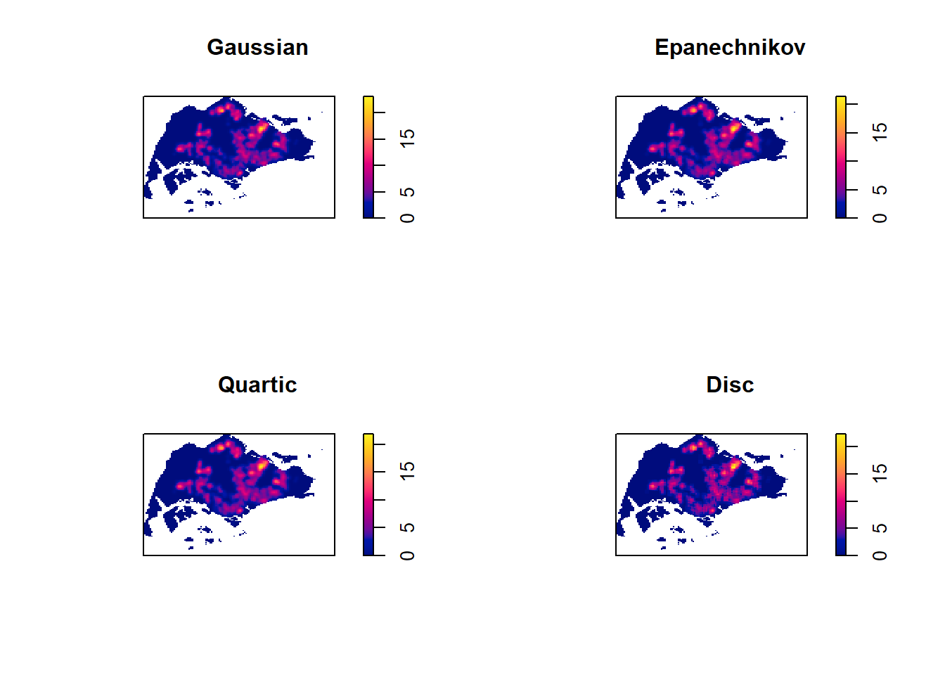
Fixed and Adaptive KDE
Fixed Bandwidth
kde_childcareSG_600 <- density(childcareSG_ppp.km, sigma=0.6, edge=TRUE, kernel="gaussian")
plot(kde_childcareSG_600)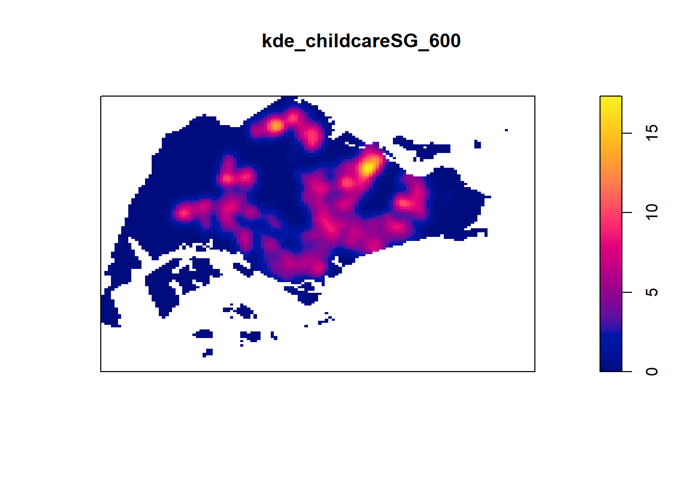
Adaptive Bandwidth
kde_childcareSG_adaptive <- adaptive.density(childcareSG_ppp.km, method="kernel")
plot(kde_childcareSG_adaptive)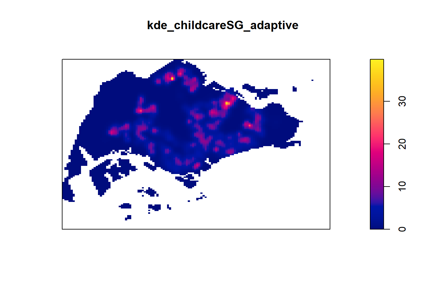
par(mfrow=c(1,2))
plot(kde_childcareSG.bw, main = "Fixed bandwidth")
plot(kde_childcareSG_adaptive, main = "Adaptive bandwidth")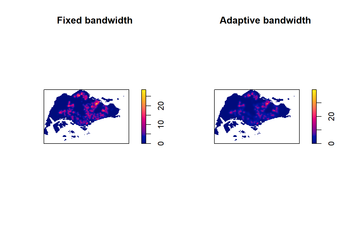
Converting KDE output into grid object
gridded_kde_childcareSG_bw <- as.SpatialGridDataFrame.im(kde_childcareSG.bw)
spplot(gridded_kde_childcareSG_bw)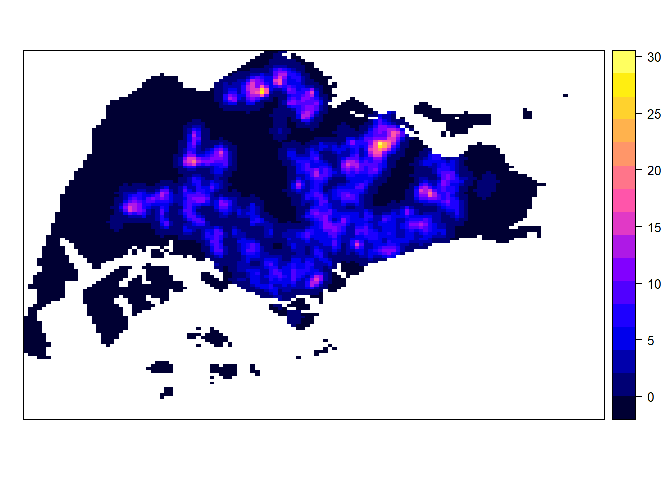
Converting into raster
kde_childcareSG_bw_raster <- raster(gridded_kde_childcareSG_bw)
kde_childcareSG_bw_rasterclass : RasterLayer
dimensions : 128, 128, 16384 (nrow, ncol, ncell)
resolution : 0.4170614, 0.2647348 (x, y)
extent : 2.663926, 56.04779, 16.35798, 50.24403 (xmin, xmax, ymin, ymax)
crs : NA
source : memory
names : v
values : -8.476185e-15, 28.51831 (min, max)Assigning projection systems
projection(kde_childcareSG_bw_raster) <- CRS("+init=EPSG:3414")
kde_childcareSG_bw_rasterclass : RasterLayer
dimensions : 128, 128, 16384 (nrow, ncol, ncell)
resolution : 0.4170614, 0.2647348 (x, y)
extent : 2.663926, 56.04779, 16.35798, 50.24403 (xmin, xmax, ymin, ymax)
crs : +init=EPSG:3414
source : memory
names : v
values : -8.476185e-15, 28.51831 (min, max)Plot in tmap
tm_shape(kde_childcareSG_bw_raster) +
tm_raster("v") +
tm_layout(legend.position = c("right", "bottom"), frame = FALSE)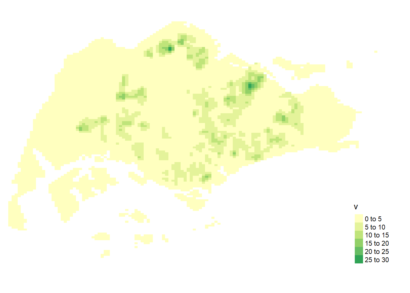
Comparing spatial point patterns using KDE
Extracting study areas
pg = mpsz[mpsz@data$PLN_AREA_N == "PUNGGOL",]
tm = mpsz[mpsz@data$PLN_AREA_N == "TAMPINES",]
ck = mpsz[mpsz@data$PLN_AREA_N == "CHOA CHU KANG",]
jw = mpsz[mpsz@data$PLN_AREA_N == "JURONG WEST",]Plotting target planning areas
par(mfrow=c(2,2))
plot(pg, main = "Ponggol")
plot(tm, main = "Tampines")
plot(ck, main = "Choa Chu Kang")
plot(jw, main = "Jurong West")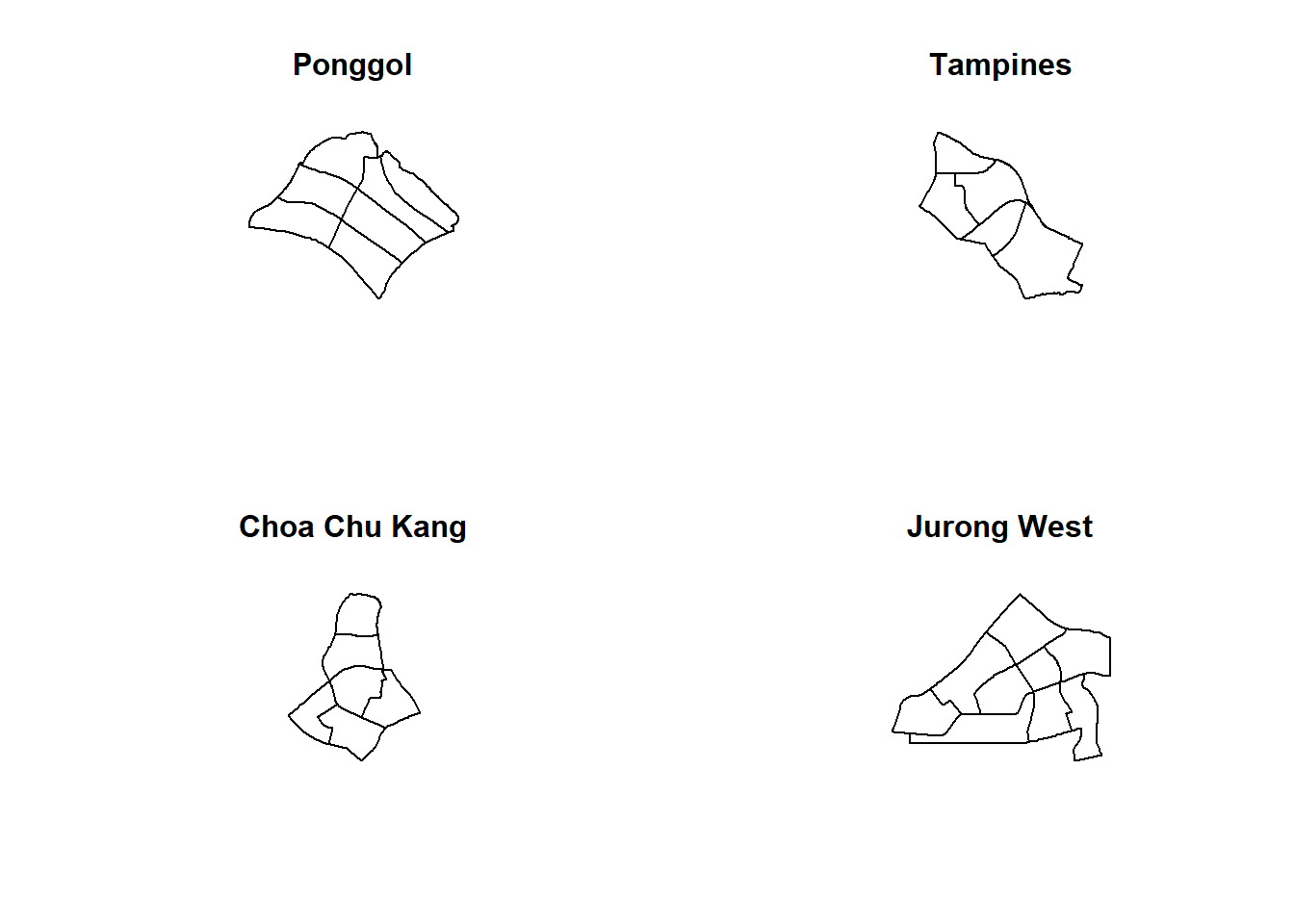
Converting into generic sp format
pg_sp = as(pg, "SpatialPolygons")
tm_sp = as(tm, "SpatialPolygons")
ck_sp = as(ck, "SpatialPolygons")
jw_sp = as(jw, "SpatialPolygons")Creating owin object
pg_owin = as(pg_sp, "owin")
tm_owin = as(tm_sp, "owin")
ck_owin = as(ck_sp, "owin")
jw_owin = as(jw_sp, "owin")Combining childcare points and the study area
childcare_pg_ppp = childcare_ppp_jit[pg_owin]
childcare_tm_ppp = childcare_ppp_jit[tm_owin]
childcare_ck_ppp = childcare_ppp_jit[ck_owin]
childcare_jw_ppp = childcare_ppp_jit[jw_owin]childcare_pg_ppp.km = rescale(childcare_pg_ppp, 1000, "km")
childcare_tm_ppp.km = rescale(childcare_tm_ppp, 1000, "km")
childcare_ck_ppp.km = rescale(childcare_ck_ppp, 1000, "km")
childcare_jw_ppp.km = rescale(childcare_jw_ppp, 1000, "km")par(mfrow=c(2,2))
plot(childcare_pg_ppp.km, main="Punggol")
plot(childcare_tm_ppp.km, main="Tampines")
plot(childcare_ck_ppp.km, main="Choa Chu Kang")
plot(childcare_jw_ppp.km, main="Jurong West")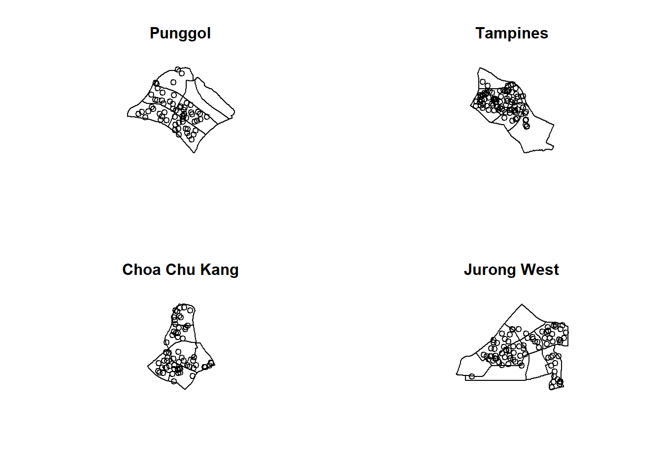
Computing KDE
par(mfrow=c(2,2))
plot(density(childcare_pg_ppp.km,
sigma=bw.diggle,
edge=TRUE,
kernel="gaussian"),
main="Punggol")
plot(density(childcare_tm_ppp.km,
sigma=bw.diggle,
edge=TRUE,
kernel="gaussian"),
main="Tempines")
plot(density(childcare_ck_ppp.km,
sigma=bw.diggle,
edge=TRUE,
kernel="gaussian"),
main="Choa Chu Kang")
plot(density(childcare_jw_ppp.km,
sigma=bw.diggle,
edge=TRUE,
kernel="gaussian"),
main="JUrong West")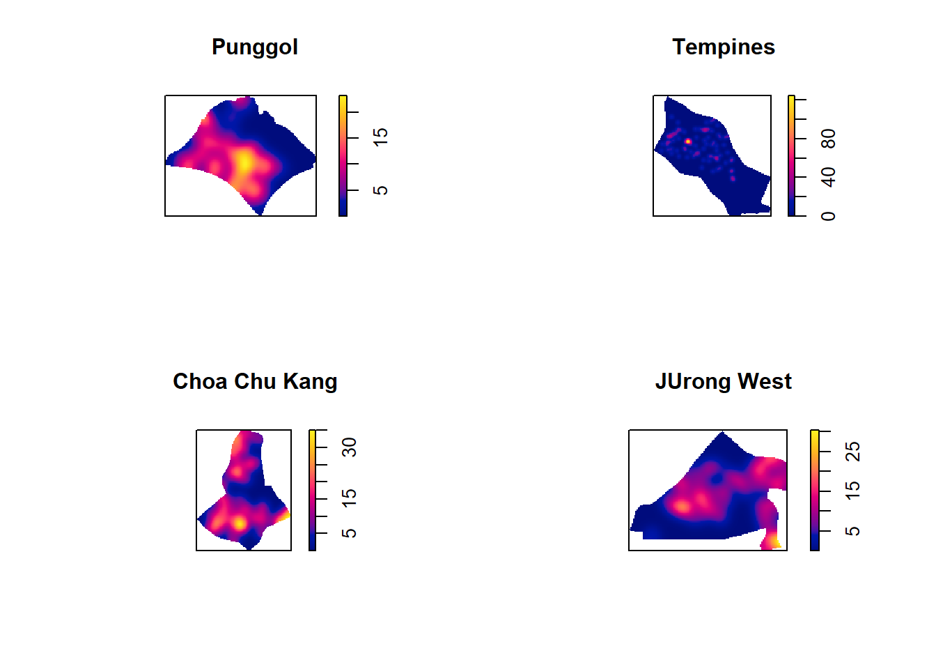
Fixed bandwidth KDE
par(mfrow=c(2,2))
plot(density(childcare_ck_ppp.km,
sigma=0.25,
edge=TRUE,
kernel="gaussian"),
main="Chou Chu Kang")
plot(density(childcare_jw_ppp.km,
sigma=0.25,
edge=TRUE,
kernel="gaussian"),
main="JUrong West")
plot(density(childcare_pg_ppp.km,
sigma=0.25,
edge=TRUE,
kernel="gaussian"),
main="Punggol")
plot(density(childcare_tm_ppp.km,
sigma=0.25,
edge=TRUE,
kernel="gaussian"),
main="Tampines")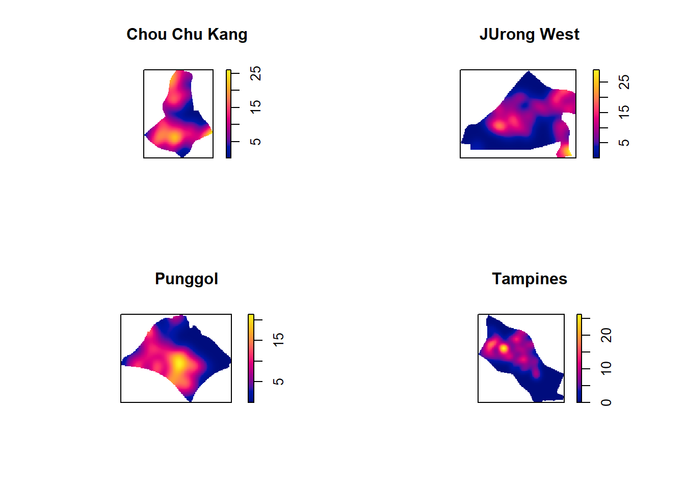
Nearest Neighbors Analysis
Clark and Evans Test
clarkevans.test(childcareSG_ppp,
correction="none",
clipregion="sg_owin",
alternative=c("clustered"),
nsim=99)
Clark-Evans test
No edge correction
Monte Carlo test based on 99 simulations of CSR with fixed n
data: childcareSG_ppp
R = 0.54756, p-value = 0.01
alternative hypothesis: clustered (R < 1)Choa Chu Kang
clarkevans.test(childcare_ck_ppp,
correction="none",
clipregion=NULL,
alternative=c("two.sided"),
nsim=999)
Clark-Evans test
No edge correction
Monte Carlo test based on 999 simulations of CSR with fixed n
data: childcare_ck_ppp
R = 0.95476, p-value = 0.132
alternative hypothesis: two-sidedTampines
clarkevans.test(childcare_tm_ppp,
correction="none",
clipregion=NULL,
alternative=c("two.sided"),
nsim=999)
Clark-Evans test
No edge correction
Monte Carlo test based on 999 simulations of CSR with fixed n
data: childcare_tm_ppp
R = 0.799, p-value = 0.002
alternative hypothesis: two-sidedSecond-order Spatial Point Patterns (Hands-On Exercise 5)
G-Function
Choa Chu Kang
Computing G-function estimation
G_CK = Gest(childcare_ck_ppp, correction = "border")
plot(G_CK, xlim=c(0,500))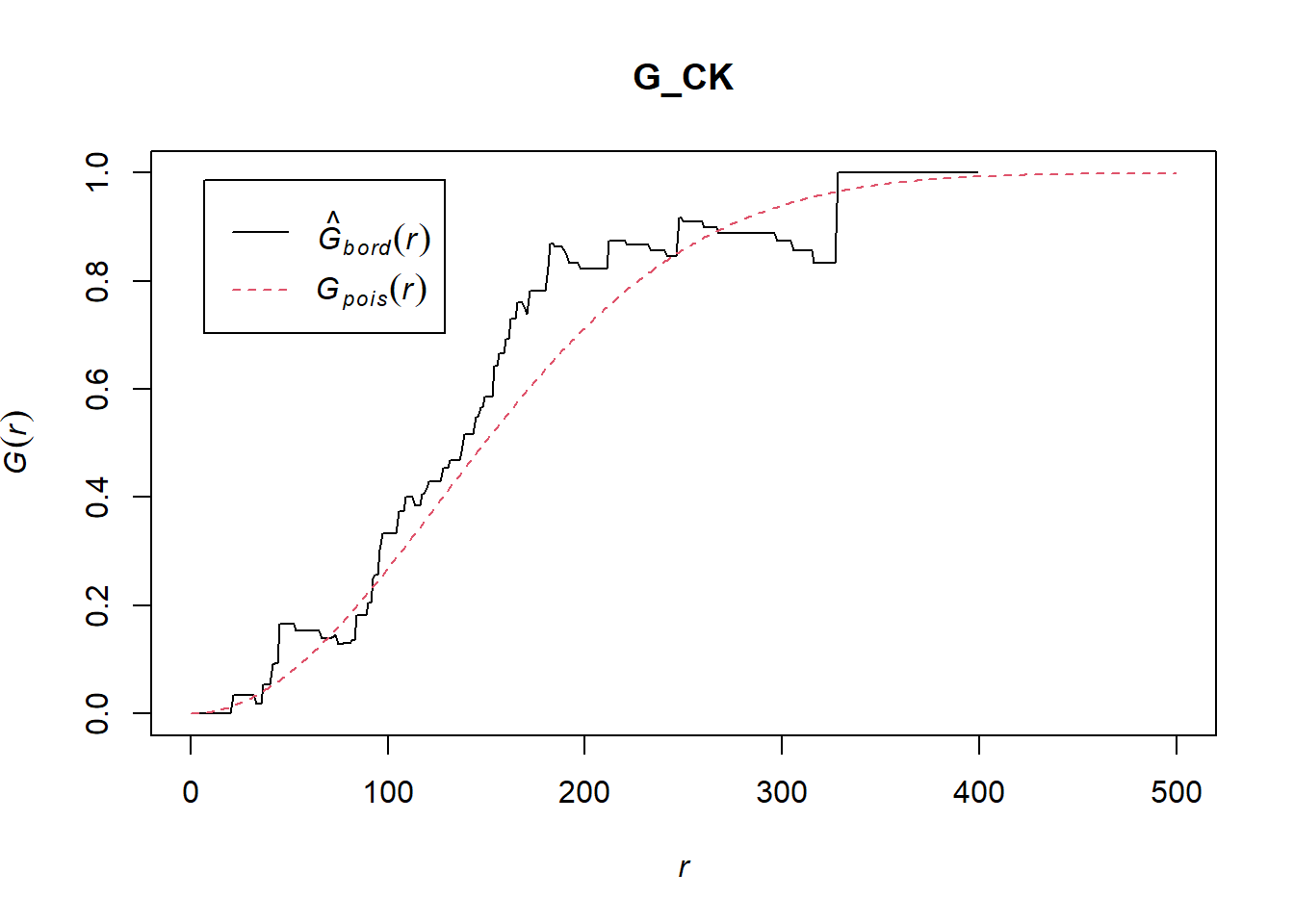
Performing Complete Spatial Randomness Test
Hypothesis test
Ho = The distribution of childcare services at Choa Chu Kang are randomly distributed
H1 = The distribution of childcare services at Choa Chu Kang are not randomly distributed
Ho rejected if p-value smaller than alpha = 0.001
G_CK.csr <- envelope(childcare_ck_ppp, Gest, nsim = 999)Generating 999 simulations of CSR ...
1, 2, 3, ......10.........20.........30.........40.........50.........60........
.70.........80.........90.........100.........110.........120.........130......
...140.........150.........160.........170.........180.........190.........200....
.....210.........220.........230.........240.........250.........260.........270..
.......280.........290.........300.........310.........320.........330.........340
.........350.........360.........370.........380.........390.........400........
.410.........420.........430.........440.........450.........460.........470......
...480.........490.........500.........510.........520.........530.........540....
.....550.........560.........570.........580.........590.........600.........610..
.......620.........630.........640.........650.........660.........670.........680
.........690.........700.........710.........720.........730.........740........
.750.........760.........770.........780.........790.........800.........810......
...820.........830.........840.........850.........860.........870.........880....
.....890.........900.........910.........920.........930.........940.........950..
.......960.........970.........980.........990........ 999.
Done.plot(G_CK.csr)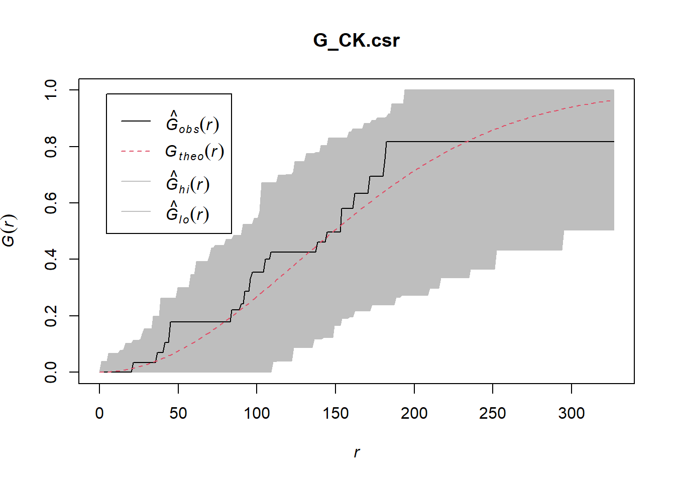
Tampines
Computing G-function estimation
G_tm = Gest(childcare_tm_ppp, correction = "best")
plot(G_tm)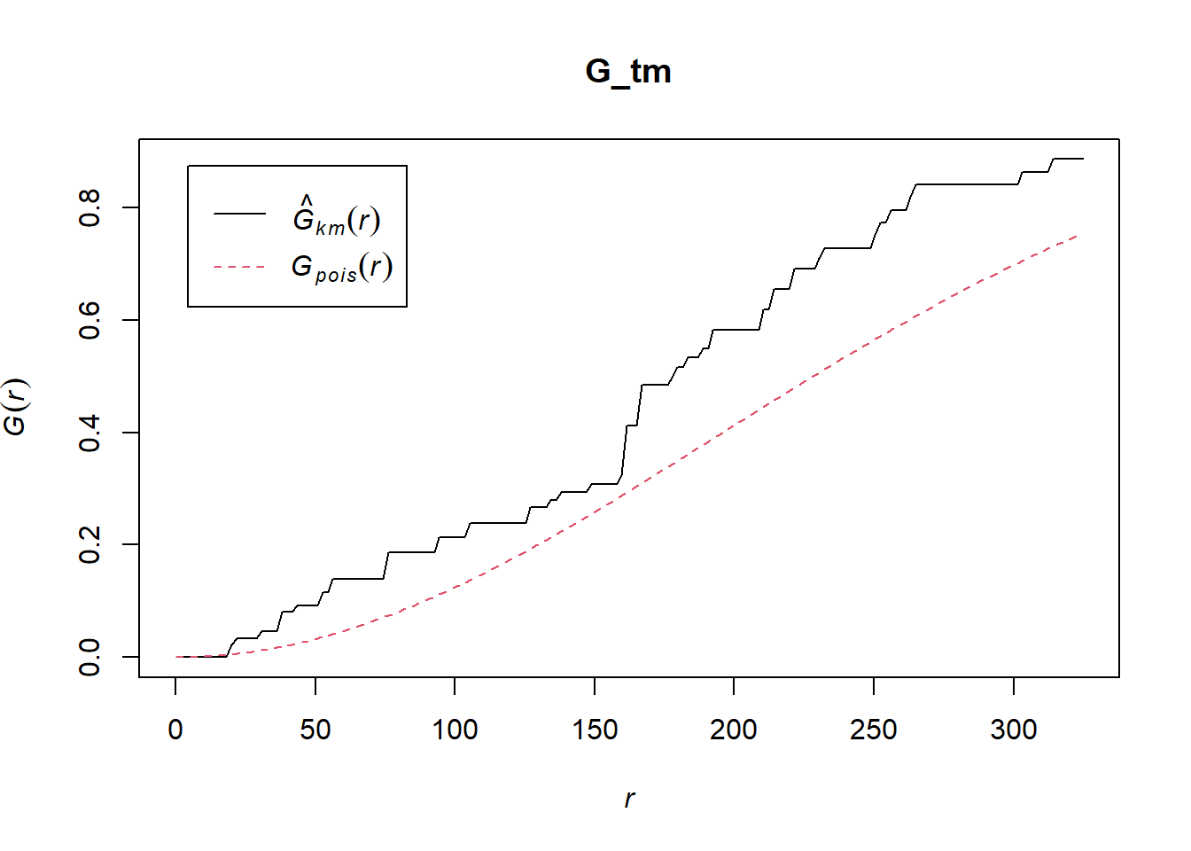
Spatial Randomness test
G_tm.csr <- envelope(childcare_tm_ppp, Gest, correction = "all", nsim = 999)Generating 999 simulations of CSR ...
1, 2, 3, ......10.........20.........30.........40.........50.........60........
.70.........80.........90.........100.........110.........120.........130......
...140.........150.........160.........170.........180.........190.........200....
.....210.........220.........230.........240.........250.........260.........270..
.......280.........290.........300.........310.........320.........330.........340
.........350.........360.........370.........380.........390.........400........
.410.........420.........430.........440.........450.........460.........470......
...480.........490.........500.........510.........520.........530.........540....
.....550.........560.........570.........580.........590.........600.........610..
.......620.........630.........640.........650.........660.........670.........680
.........690.........700.........710.........720.........730.........740........
.750.........760.........770.........780.........790.........800.........810......
...820.........830.........840.........850.........860.........870.........880....
.....890.........900.........910.........920.........930.........940.........950..
.......960.........970.........980.........990........ 999.
Done.plot(G_tm.csr)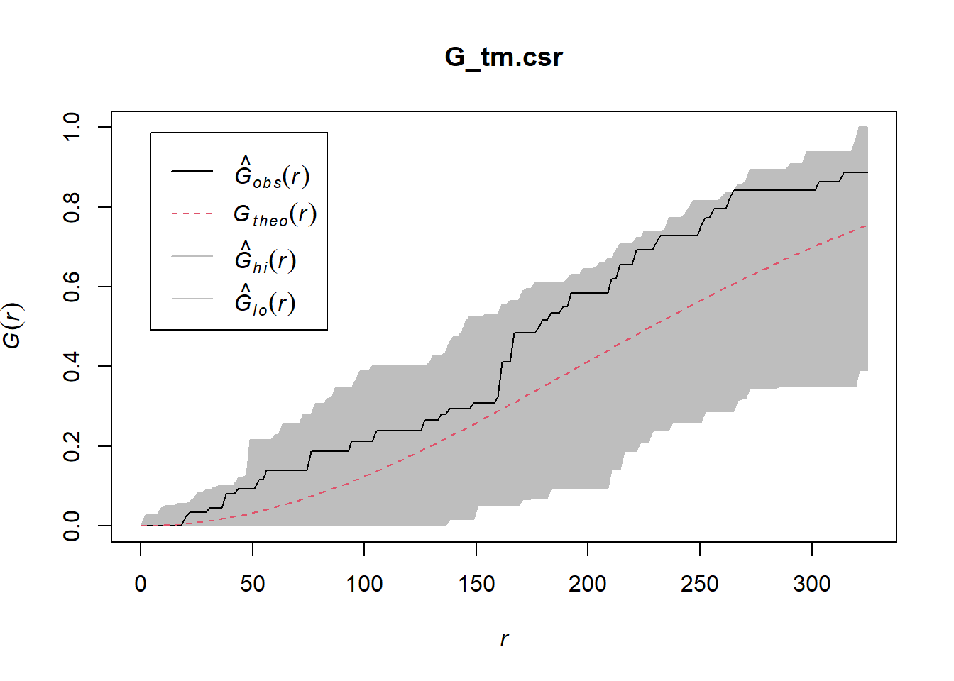
F-Function
Choa Chu Kang
Computing F-function estimation
F_CK = Fest(childcare_ck_ppp)
plot(F_CK)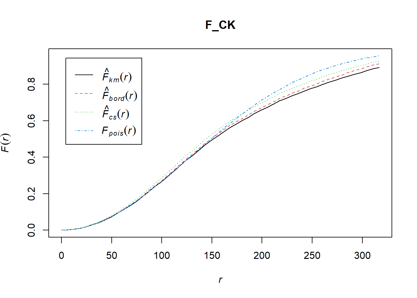
Performing complete Spatial Randomness Test
F_CK.csr <- envelope(childcare_ck_ppp, Fest, nsim = 999)Generating 999 simulations of CSR ...
1, 2, 3, ......10.........20.........30.........40.........50.........60........
.70.........80.........90.........100.........110.........120.........130......
...140.........150.........160.........170.........180.........190.........200....
.....210.........220.........230.........240.........250.........260.........270..
.......280.........290.........300.........310.........320.........330.........340
.........350.........360.........370.........380.........390.........400........
.410.........420.........430.........440.........450.........460.........470......
...480.........490.........500.........510.........520.........530.........540....
.....550.........560.........570.........580.........590.........600.........610..
.......620.........630.........640.........650.........660.........670.........680
.........690.........700.........710.........720.........730.........740........
.750.........760.........770.........780.........790.........800.........810......
...820.........830.........840.........850.........860.........870.........880....
.....890.........900.........910.........920.........930.........940.........950..
.......960.........970.........980.........990........ 999.
Done.plot(F_CK.csr)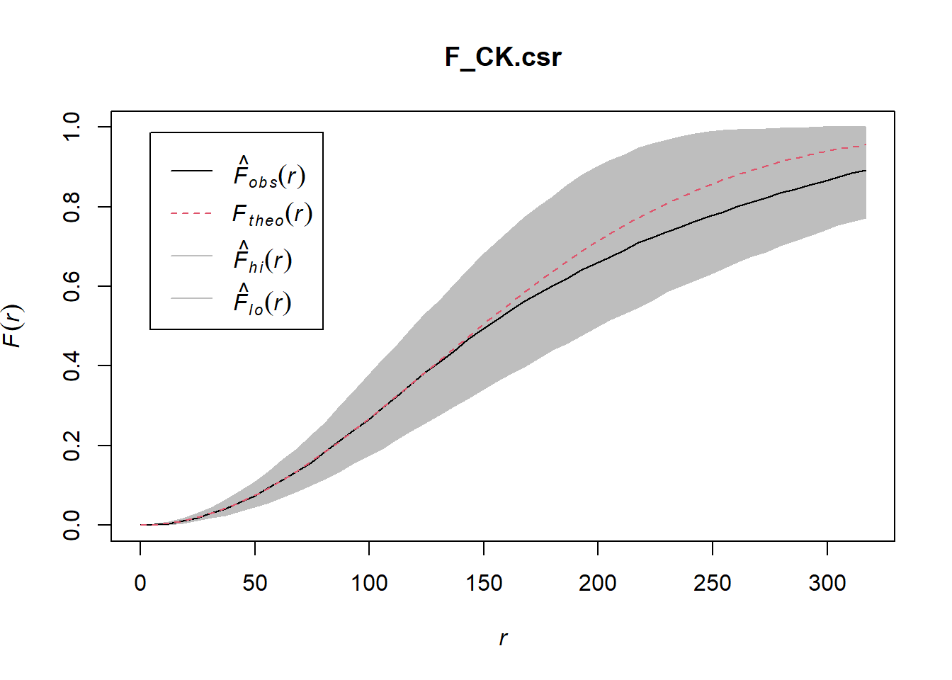
Tampines
Computing F-function estimation
F_tm = Fest(childcare_tm_ppp, correction = "best")
plot(F_tm)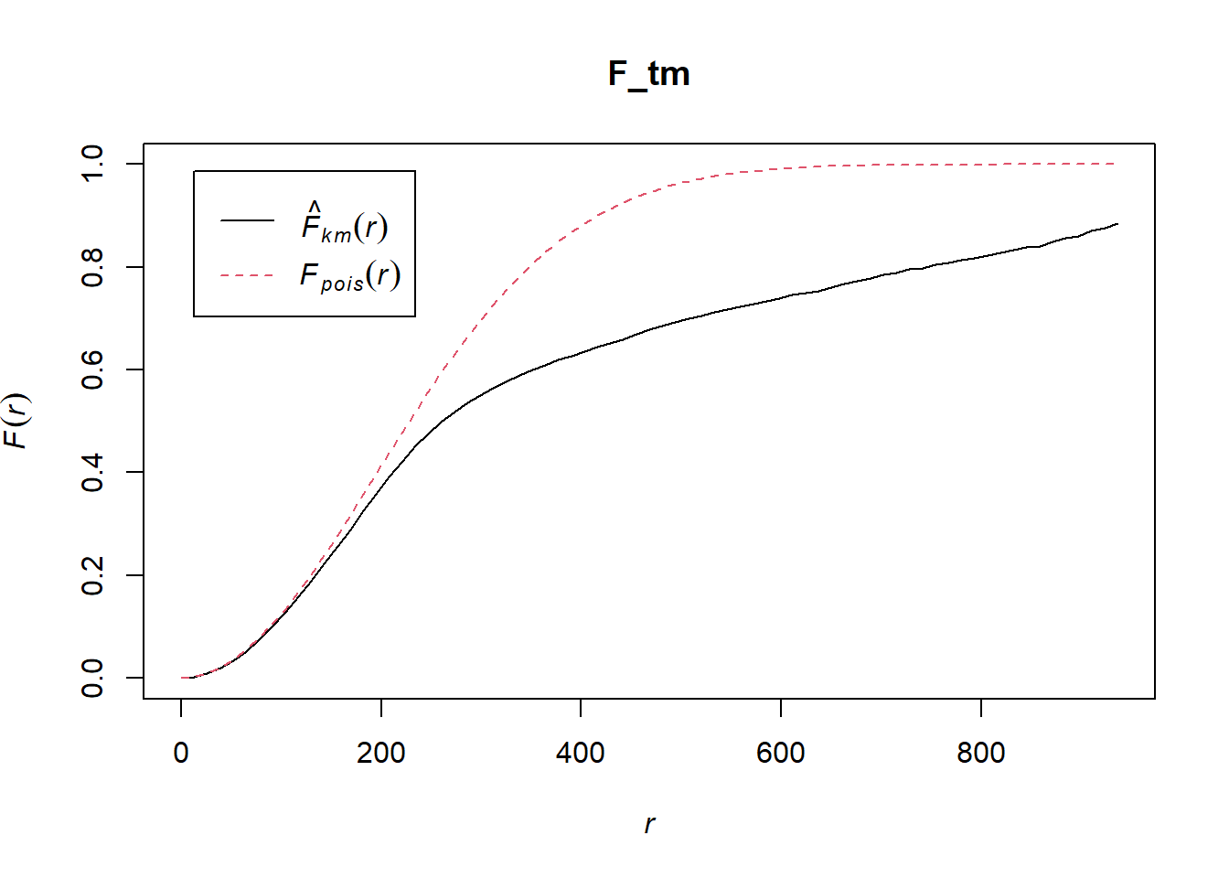
Performing complete Spatial Randomness Test
F_tm.csr <- envelope(childcare_tm_ppp, Fest, correction = "all", nsim = 999)Generating 999 simulations of CSR ...
1, 2, 3, ......10.........20.........30.........40.........50.........60........
.70.........80.........90.........100.........110.........120.........130......
...140.........150.........160.........170.........180.........190.........200....
.....210.........220.........230.........240.........250.........260.........270..
.......280.........290.........300.........310.........320.........330.........340
.........350.........360.........370.........380.........390.........400........
.410.........420.........430.........440.........450.........460.........470......
...480.........490.........500.........510.........520.........530.........540....
.....550.........560.........570.........580.........590.........600.........610..
.......620.........630.........640.........650.........660.........670.........680
.........690.........700.........710.........720.........730.........740........
.750.........760.........770.........780.........790.........800.........810......
...820.........830.........840.........850.........860.........870.........880....
.....890.........900.........910.........920.........930.........940.........950..
.......960.........970.........980.........990........ 999.
Done.plot(F_tm.csr)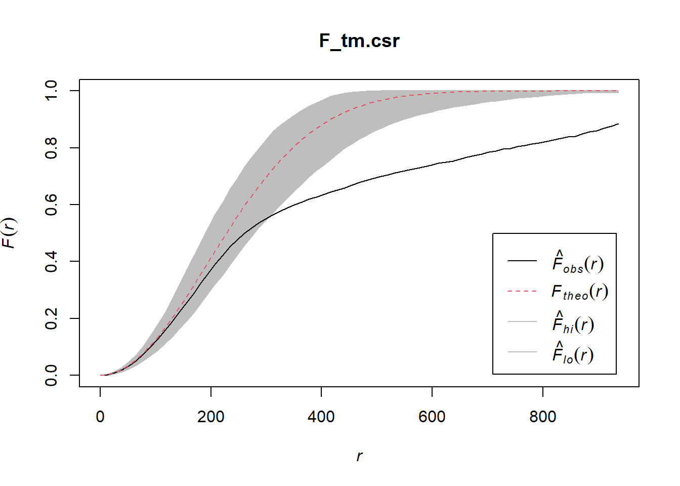
K-Function
Choa Chu Kang
Computing K-function estimate
K_ck = Kest(childcare_ck_ppp, correction = "Ripley")
plot(K_ck, . -r ~ r, ylab= "K(d)-r", xlab = "d(m)")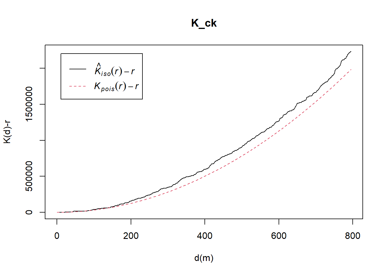
Performing complete Spatial Randomness Test
K_ck.csr <- envelope(childcare_ck_ppp, Kest, nsim = 99, rank = 1, glocal=TRUE)Generating 99 simulations of CSR ...
1, 2, 3, 4, 5, 6, 7, 8, 9, 10, 11, 12, 13, 14, 15, 16, 17, 18, 19, 20, 21, 22, 23, 24, 25, 26, 27, 28, 29, 30, 31, 32, 33, 34, 35, 36, 37, 38, 39, 40,
41, 42, 43, 44, 45, 46, 47, 48, 49, 50, 51, 52, 53, 54, 55, 56, 57, 58, 59, 60, 61, 62, 63, 64, 65, 66, 67, 68, 69, 70, 71, 72, 73, 74, 75, 76, 77, 78, 79, 80,
81, 82, 83, 84, 85, 86, 87, 88, 89, 90, 91, 92, 93, 94, 95, 96, 97, 98, 99.
Done.plot(K_ck.csr, . - r ~ r, xlab="d", ylab="K(d)-r")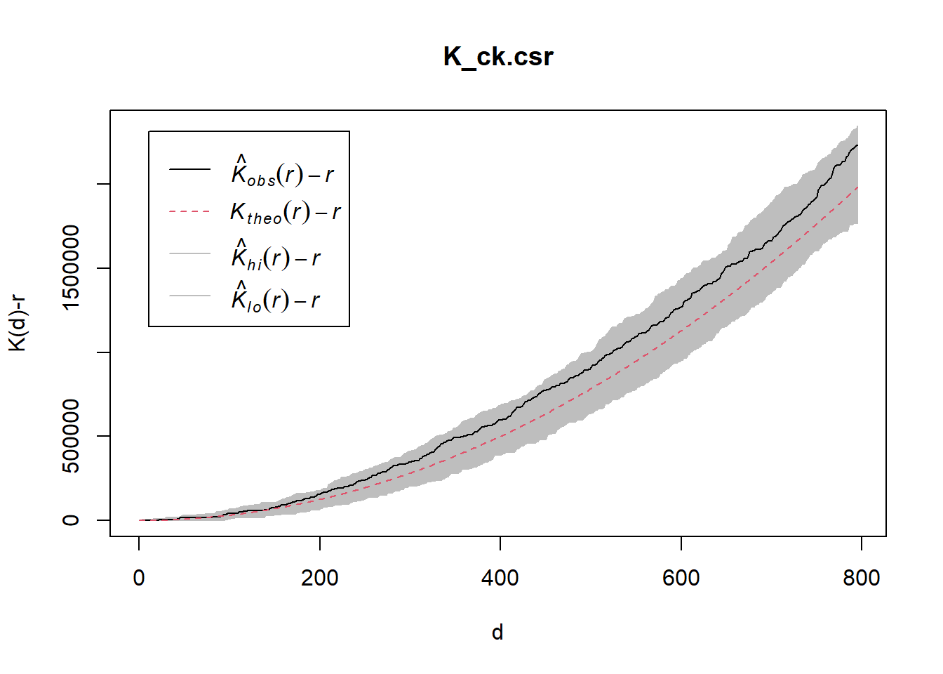
Tampines
Computing K-function estimation
K_tm = Kest(childcare_tm_ppp, correction = "Ripley")
plot(K_tm, . -r ~ r,
ylab= "K(d)-r", xlab = "d(m)",
xlim=c(0,1000))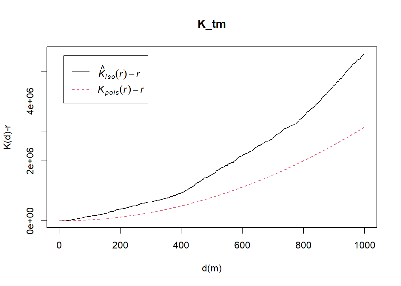
Performing complete Spatial Randomness Test
K_tm.csr <- envelope(childcare_tm_ppp, Kest, nsim = 99, rank = 1, glocal=TRUE)Generating 99 simulations of CSR ...
1, 2, 3, 4, 5, 6, 7, 8, 9, 10, 11, 12, 13, 14, 15, 16, 17, 18, 19, 20, 21, 22, 23, 24, 25, 26, 27, 28, 29, 30, 31, 32, 33, 34, 35, 36, 37, 38, 39, 40,
41, 42, 43, 44, 45, 46, 47, 48, 49, 50, 51, 52, 53, 54, 55, 56, 57, 58, 59, 60, 61, 62, 63, 64, 65, 66, 67, 68, 69, 70, 71, 72, 73, 74, 75, 76, 77, 78, 79, 80,
81, 82, 83, 84, 85, 86, 87, 88, 89, 90, 91, 92, 93, 94, 95, 96, 97, 98, 99.
Done.plot(K_tm.csr, . - r ~ r,
xlab="d", ylab="K(d)-r", xlim=c(0,500))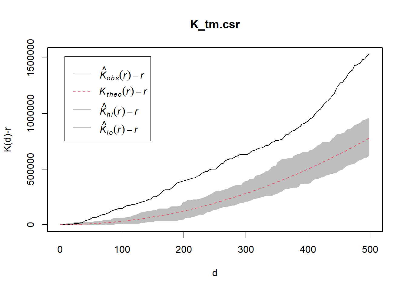
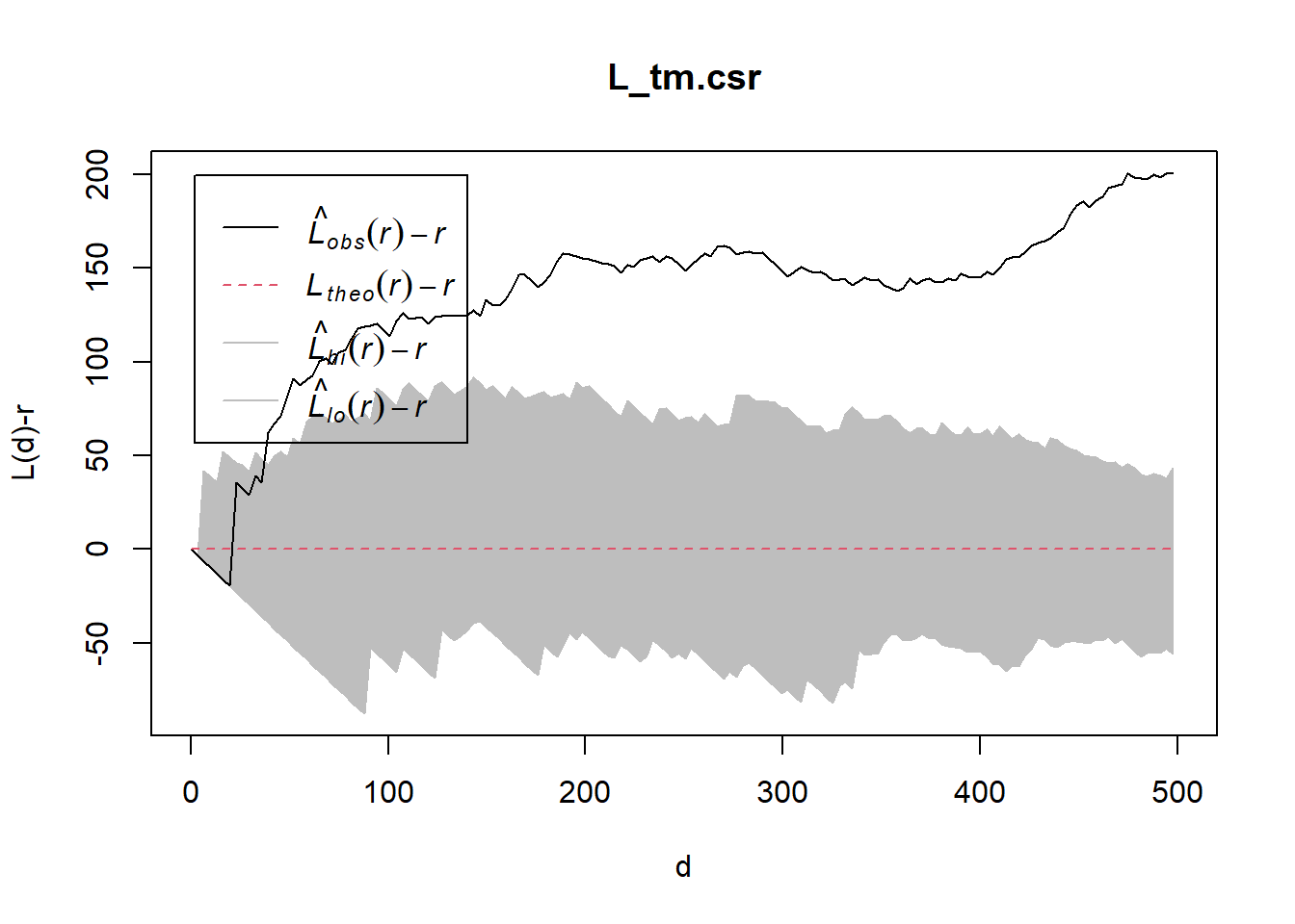
L-Function
Choa Chu Kang
Computing L Function estimation
L_ck = Lest(childcare_ck_ppp, correction = "Ripley")
plot(L_ck, . -r ~ r,
ylab= "L(d)-r", xlab = "d(m)")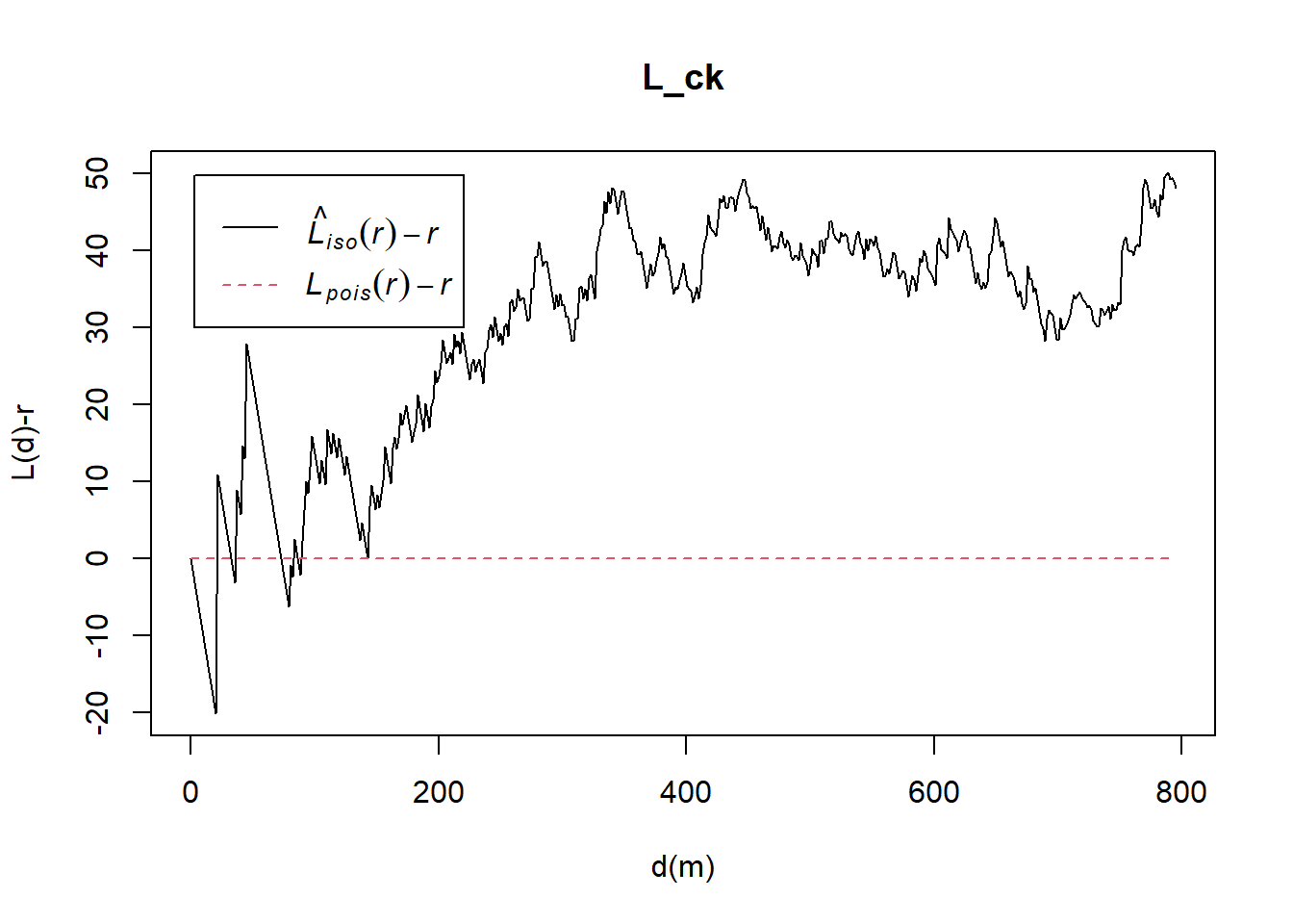
Performing complete Spatial Randomness Test
L_ck.csr <- envelope(childcare_ck_ppp, Lest, nsim = 99, rank = 1, glocal=TRUE)Generating 99 simulations of CSR ...
1, 2, 3, 4, 5, 6, 7, 8, 9, 10, 11, 12, 13, 14, 15, 16, 17, 18, 19, 20, 21, 22, 23, 24, 25, 26, 27, 28, 29, 30, 31, 32, 33, 34, 35, 36, 37, 38, 39, 40,
41, 42, 43, 44, 45, 46, 47, 48, 49, 50, 51, 52, 53, 54, 55, 56, 57, 58, 59, 60, 61, 62, 63, 64, 65, 66, 67, 68, 69, 70, 71, 72, 73, 74, 75, 76, 77, 78, 79, 80,
81, 82, 83, 84, 85, 86, 87, 88, 89, 90, 91, 92, 93, 94, 95, 96, 97, 98, 99.
Done.plot(L_ck.csr, . - r ~ r, xlab="d", ylab="L(d)-r")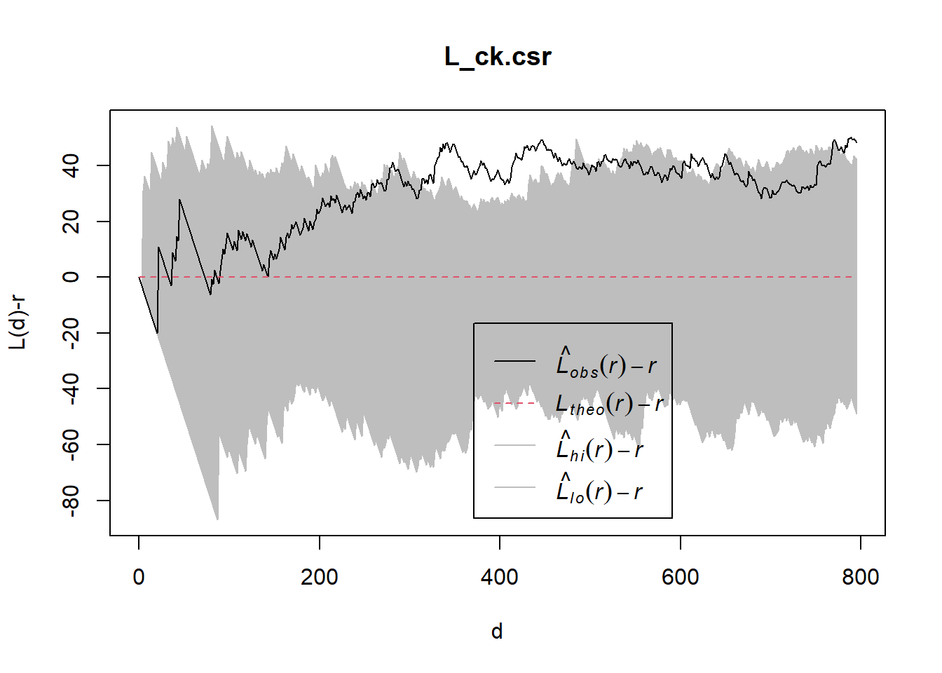
Tampines
Computing L-function estimate
L_tm = Lest(childcare_tm_ppp, correction = "Ripley")
plot(L_tm, . -r ~ r,
ylab= "L(d)-r", xlab = "d(m)",
xlim=c(0,1000))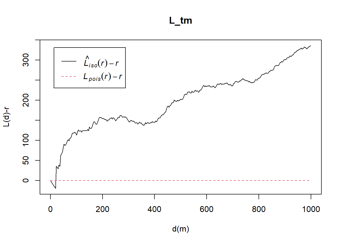
Performing complete Spatial Randomness Test
L_tm.csr <- envelope(childcare_tm_ppp, Lest, nsim = 99, rank = 1, glocal=TRUE)Generating 99 simulations of CSR ...
1, 2, 3, 4, 5, 6, 7, 8, 9, 10, 11, 12, 13, 14, 15, 16, 17, 18, 19, 20, 21, 22, 23, 24, 25, 26, 27, 28, 29, 30, 31, 32, 33, 34, 35, 36, 37, 38, 39, 40,
41, 42, 43, 44, 45, 46, 47, 48, 49, 50, 51, 52, 53, 54, 55, 56, 57, 58, 59, 60, 61, 62, 63, 64, 65, 66, 67, 68, 69, 70, 71, 72, 73, 74, 75, 76, 77, 78, 79, 80,
81, 82, 83, 84, 85, 86, 87, 88, 89, 90, 91, 92, 93, 94, 95, 96, 97, 98, 99.
Done.plot(L_tm.csr, . - r ~ r,
xlab="d", ylab="L(d)-r", xlim=c(0,500))