In-Class Exercise 3: Thematic and Analytical Mapping

Import Packages

pacman::p_load(sf, tidyverse, tmap)

Import Data

We will be reusing ICE2’s RDS of nga_combined.

NGA_wp <- read_rds("../chapter-02/data/rds/NGA_wp.rds")

glimpse(NGA_wp)

Rows: 774
Columns: 9
$ ADM2_EN           <chr> "Aba North", "Aba South", "Abadam", "Abaji", "Abak",…
$ ADM2_PCODE        <chr> "NG001001", "NG001002", "NG008001", "NG015001", "NG0…
$ ADM1_EN           <chr> "Abia", "Abia", "Borno", "Federal Capital Territory"…
$ ADM1_PCODE        <chr> "NG001", "NG001", "NG008", "NG015", "NG003", "NG011"…
$ geometry          <MULTIPOLYGON [m]> MULTIPOLYGON (((548795.5 11..., MULTIPO…
$ WP_Functional     <int> 7, 29, 0, 23, 23, 82, 16, 72, 79, 18, 25, 54, 28, 55…
$ WP_Non_Functional <int> 9, 35, 0, 34, 25, 42, 15, 33, 62, 26, 13, 73, 35, 36…
$ WP_Unknown        <int> 1, 7, 0, 0, 0, 109, 3, 14, 11, 22, 1, 8, 0, 37, 88, …
$ WP_Total          <int> 17, 71, 0, 57, 48, 233, 34, 119, 152, 66, 39, 135, 6…

Choropleth Mapping

p1 <- tm_shape(NGA_wp) +
  tm_fill("WP_Functional",
          n = 10, # 10 classes
          style = "equal",
          palette = "Blues") +
  tm_borders(lwd = 0.1,
             alpha = 1) +
  tm_layout(main.title = "Distribution of functional water points",
            legend.outside = FALSE)
p1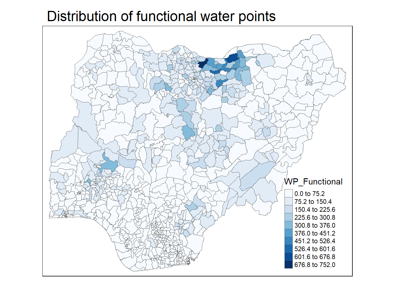

p2 <- tm_shape(NGA_wp) +
  tm_fill("WP_Total",
          n = 10, # 10 classes
          style = "equal",
          palette = "Blues") +
  tm_borders(lwd = 0.1,
             alpha = 1) +
  tm_layout(main.title = "Distribution of total water points",
            legend.outside = FALSE)

Small multiples

tmap_arrange(p2, p1, nrow=1)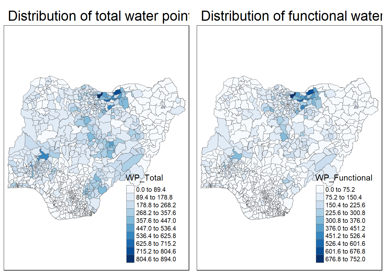

Choropleth Map for Rates

NGA_wp <- NGA_wp %>%
  mutate(`WP_Functional_Proportion` = `WP_Functional`/`WP_Total`,
         `WP_Non_Functional_Proportion` = `WP_Non_Functional`/`WP_Total`)

Plotting map of rate

p3 <- tm_shape(NGA_wp) +
  tm_fill("WP_Functional_Proportion",
          n = 10, # 10 classes
          title = "Functional WP Proportion",
          style = "equal",
          palette = "Blues") +
  tm_borders(lwd = 0.1,
             alpha = 1) +
  tm_layout(main.title = "Rate Map of Functional Water Points",
            legend.outside = TRUE)
p3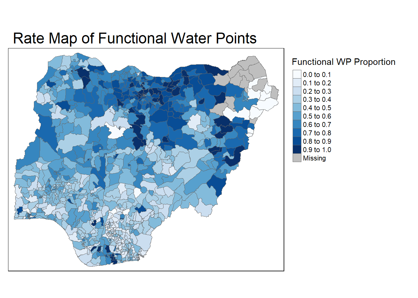

Percentile Map

Special type of quantile map with six specific categories: 0-1%, 1-10%, 10-50%, 50-90%, 90-99%, and 99-100%. We need to create a classification scheme using breakpoints that are derived by means of the quantile command, passing an explicit vector of cumulative probabilities as c(0, .01, .1, .5, .9, .99). Begin and endpoint need to be included.

Data Preparations

Drop NA values

NGA_wp <- NGA_wp %>% drop_na()

Create customised classification and extract values

percent <- c(0, .01, .1, .5, .9, .99)
var <- NGA_wp["WP_Functional_Proportion"] %>%
  st_set_geometry(NULL) # need to drop the geometric field
quantile(var[,1], percent)

       0%        1%       10%       50%       90%       99% 
0.0000000 0.0000000 0.2169811 0.4791667 0.8611111 1.0000000 

Utility Functions

Create get.var function to generalise the customised classification steps

• Arguments:

  • vname: variable name that you want to plot (as character, in quotes)

  • df: name of sf data frame

• Returns:

  • v: vector with values (without a column name)

get.var <- function(vname, df) {
  v <- df[vname] %>%
    st_set_geometry(NULL)
  v <- unname(v[,1])
  return(v)
}

Create percentmap function to plot the percentile map

percentmap <- function(vname, df, legtitle=NA, mtitle="Percentile Map") {
  percent <- c(0, .01, .1, .5, .9, .99)
  var <- get.var(vname, df)
  bperc <- quantile(var, percent)
  tm_shape(df) +
    tm_polygons() +
    tm_shape(df) +
    tm_fill(vname,
            title=legtitle,
            breaks=bperc,
            palette="Blues",
            labels=c("< 1%", "1-10%", "10-50%", "50-90%", "90-99%", "> 99%")) +
    tm_borders() +
    tm_layout(main.title = mtitle,
              legend.outside = TRUE,
              legend.position = c("right", "bottom"),
              title.position = c("right", "bottom"))
  
}

Plot

percentmap("WP_Functional_Proportion", NGA_wp, legtitle = "Functional Proportion")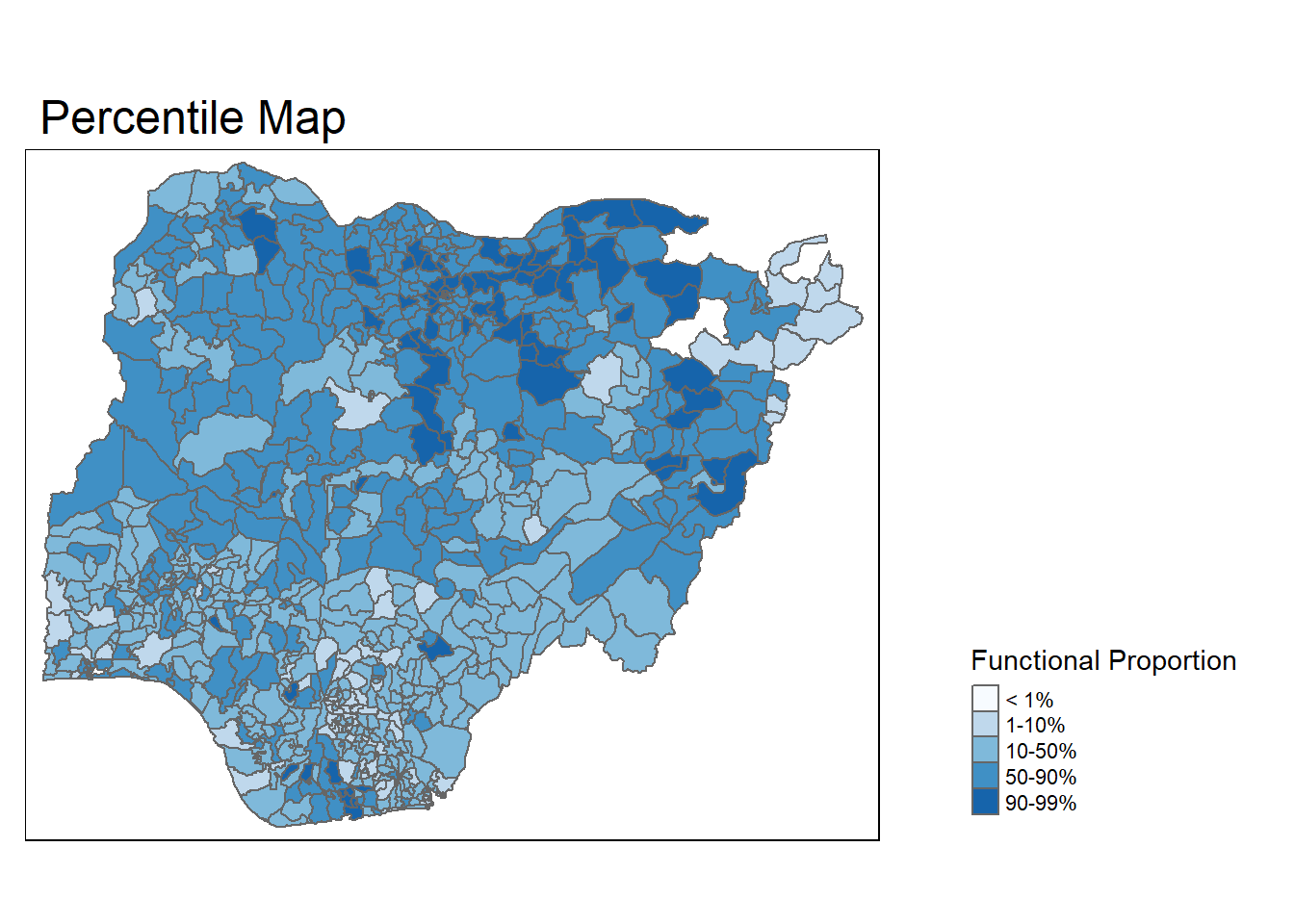

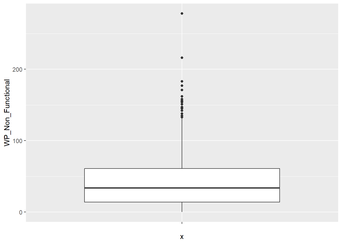
Box Plot

For visualising outliers and distribution

ggplot(data = NGA_wp, aes(x="", y=WP_Non_Functional)) +
  geom_boxplot()