pacman::p_load(sf, sfdep, tmap, tidyverse, plotly)In-Class Exercise 7: Global & Local Measures of Spatial Autocorrelation
Import Packages
Import Dataset
Geospatial
hunan <- st_read(dsn = "../chapter-06/data/geospatial",
                 layer = "Hunan")
Reading layer `Hunan' from data source
`C:\Jenpoer\IS415-GAA\In-Class-Exercises\chapter-06\data\geospatial'
using driver `ESRI Shapefile'
Simple feature collection with 88 features and 7 fields
Geometry type: POLYGON
Dimension: XY
Bounding box: xmin: 108.7831 ymin: 24.6342 xmax: 114.2544 ymax: 30.12812
Geodetic CRS: WGS 84Aspatial
hunan2012 <- read_csv("../chapter-06/data/aspatial/Hunan_2012.csv")Data Preprocessing
Combining data frame with left join
hunan_GDPPC <- left_join(hunan,hunan2012) %>%
select(1:4, 7, 15)tm_shape(hunan_GDPPC)+
tm_fill("GDPPC",
style = "quantile",
palette = "Blues",
title = "GDPPC") +
tm_layout(main.title = "Distribution of GDP per capita by district, Hunan Province",
main.title.position = "center",
main.title.size = 1,
legend.outside = TRUE,
legend.position = c("right", "bottom"),
frame = TRUE) +
tm_borders(alpha=0.5) +
tm_compass(type="8star", size = 2) +
tm_scale_bar() +
tm_grid(alpha = 0.2)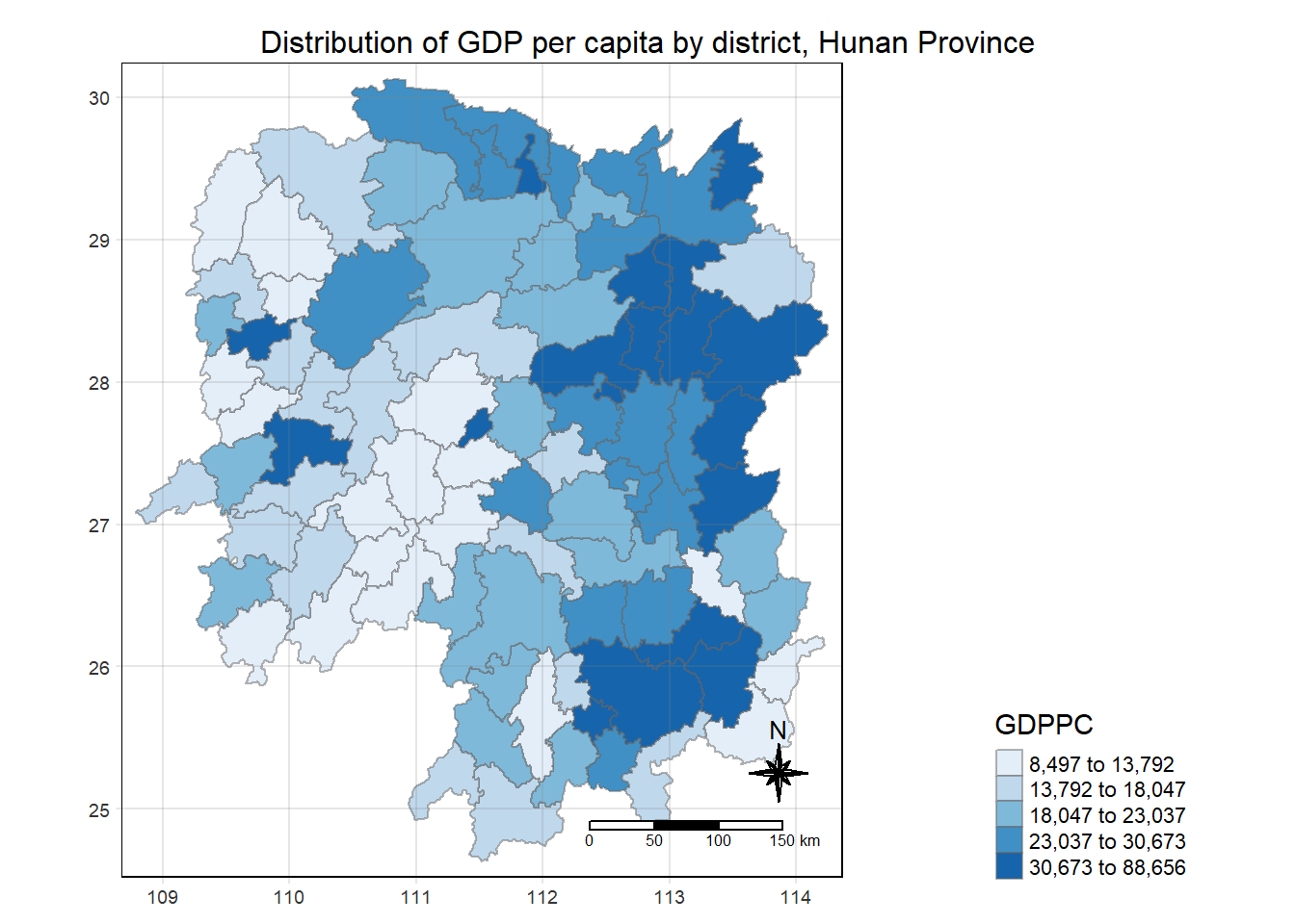
Identify Polygon Neighbors
wm_q <- hunan_GDPPC %>%
  mutate(nb = st_contiguity(geometry),
         wt = st_weights(nb, style = "W"),
         .before = 1) # put newly-created field in first column
Computing Global Moran’s I
moran1 <- global_moran(wm_q$GDPPC,
                       wm_q$nb,
                       wm_q$wt)
Perfom the Global Moran’s I test (only doing this step is sufficient)
global_moran_test(wm_q$GDPPC,
                  wm_q$nb,
                  wm_q$wt)
    Moran I test under randomisation

data:  x
weights: listw

Moran I statistic standard deviate = 4.7351, p-value = 1.095e-06
alternative hypothesis: greater
sample estimates:
Moran I statistic       Expectation          Variance
      0.300749970      -0.011494253       0.004348351
Perform Global Moran’s I permutation test
set.seed(1234)global_moran_perm(wm_q$GDPPC,
wm_q$nb,
wm_q$wt,
nsim=99)
    Monte-Carlo simulation of Moran I

data:  x
weights: listw
number of simulations + 1: 100

statistic = 0.30075, observed rank = 100, p-value < 2.2e-16
alternative hypothesis: two.sided
Computing Local Moran’s I
lisa <- wm_q %>%
  mutate(`Local_Moran` = local_moran(GDPPC, nb, wt, nsim=99),
         .before = 1) %>%
  unnest(`Local_Moran`)

lisa
Simple feature collection with 88 features and 20 fields
Geometry type: POLYGON
Dimension: XY
Bounding box: xmin: 108.7831 ymin: 24.6342 xmax: 114.2544 ymax: 30.12812
Geodetic CRS: WGS 84
# A tibble: 88 × 21
ii eii var_ii z_ii p_ii p_ii_…¹ p_fol…² skewn…³ kurtosis
<dbl> <dbl> <dbl> <dbl> <dbl> <dbl> <dbl> <dbl> <dbl>
1 -0.00147 0.00177 4.18e-4 -0.158 0.874 0.82 0.41 -0.812 0.652
2 0.0259 0.00641 1.05e-2 0.190 0.849 0.96 0.48 -1.09 1.89
3 -0.0120 -0.0374 1.02e-1 0.0796 0.937 0.76 0.38 0.824 0.0461
4 0.00102 -0.0000349 4.37e-6 0.506 0.613 0.64 0.32 1.04 1.61
5 0.0148 -0.00340 1.65e-3 0.449 0.654 0.5 0.25 1.64 3.96
6 -0.0388 -0.00339 5.45e-3 -0.480 0.631 0.82 0.41 0.614 -0.264
7 3.37 -0.198 1.41e+0 3.00 0.00266 0.08 0.04 1.46 2.74
8 1.56 -0.265 8.04e-1 2.04 0.0417 0.08 0.04 0.459 -0.519
9 4.42 0.0450 1.79e+0 3.27 0.00108 0.02 0.01 0.746 -0.00582
10 -0.399 -0.0505 8.59e-2 -1.19 0.234 0.28 0.14 -0.685 0.134
# … with 78 more rows, 12 more variables: mean <fct>, median <fct>,
# pysal <fct>, nb <nb>, wt <list>, NAME_2 <chr>, ID_3 <int>, NAME_3 <chr>,
# ENGTYPE_3 <chr>, County <chr>, GDPPC <dbl>, geometry <POLYGON [°]>, and
# abbreviated variable names ¹p_ii_sim, ²p_folded_sim, ³skewnessPlot local Moran’s I
tmap_mode("plot")
tm_shape(lisa) +
  tm_fill("ii") +
  tm_borders(alpha = 0.5)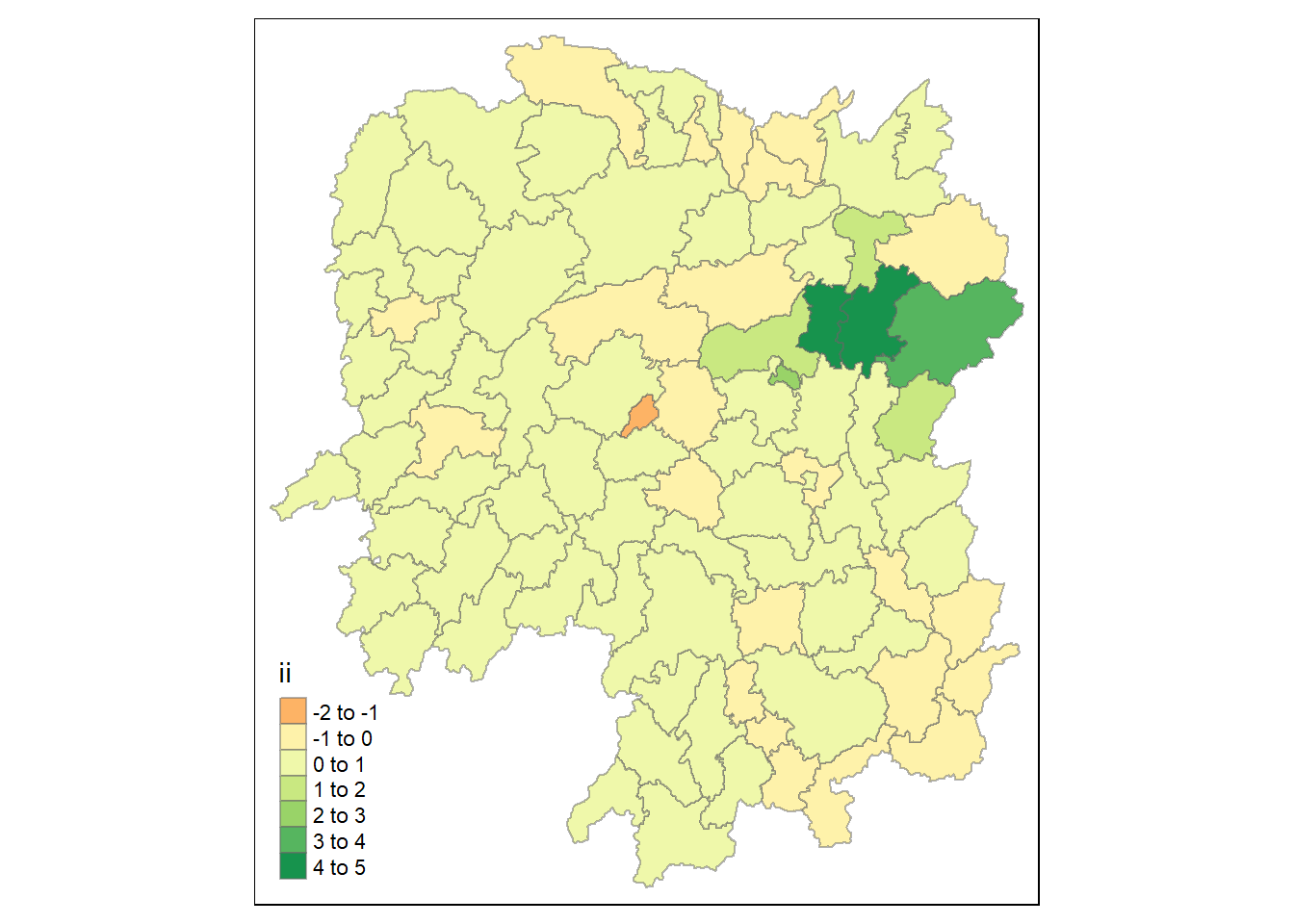
Plot p-value of local Moran’s I (but ideally, you should use the simulation values)
tmap_mode("plot")
tm_shape(lisa) +
  tm_fill("p_ii_sim") +
  tm_borders(alpha = 0.5)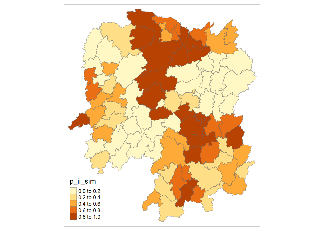
lisa_sig <- lisa %>% filter(p_ii_sim < 0.05)

tmap_mode("plot")
tm_shape(lisa) +
  tm_polygons() +
  tm_borders(alpha = 0.5) +
  tm_shape(lisa_sig) +
  tm_fill("mean") +
  tm_borders(alpha=0.5)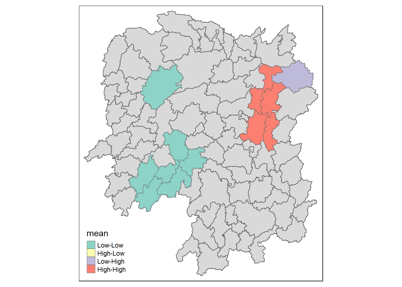
Computing Local Gi*
Include itself
HCSA <- wm_q %>%
  mutate(local_Gi = local_gstar_perm(GDPPC, nb, wt, nsim=99),
         .before = 1) %>%
  unnest(local_Gi)

HCSA
Simple feature collection with 88 features and 16 fields
Geometry type: POLYGON
Dimension: XY
Bounding box: xmin: 108.7831 ymin: 24.6342 xmax: 114.2544 ymax: 30.12812
Geodetic CRS: WGS 84
# A tibble: 88 × 17
gi_star e_gi var_gi p_value p_sim p_fol…¹ skewn…² kurto…³ nb wt
<dbl> <dbl> <dbl> <dbl> <dbl> <dbl> <dbl> <dbl> <nb> <lis>
1 -0.00567 0.0115 0.00000812 9.95e-1 0.82 0.41 1.03 1.23 <int> <dbl>
2 -0.235 0.0110 0.00000581 8.14e-1 1 0.5 0.912 1.05 <int> <dbl>
3 0.298 0.0114 0.00000776 7.65e-1 0.7 0.35 0.455 -0.732 <int> <dbl>
4 0.145 0.0121 0.0000111 8.84e-1 0.64 0.32 0.900 0.726 <int> <dbl>
5 0.356 0.0113 0.0000119 7.21e-1 0.64 0.32 1.08 1.31 <int> <dbl>
6 -0.480 0.0116 0.00000706 6.31e-1 0.82 0.41 0.364 -0.676 <int> <dbl>
7 3.66 0.0116 0.00000825 2.47e-4 0.02 0.01 0.909 0.664 <int> <dbl>
8 2.14 0.0116 0.00000714 3.26e-2 0.16 0.08 1.13 1.48 <int> <dbl>
9 4.55 0.0113 0.00000656 5.28e-6 0.02 0.01 1.36 4.14 <int> <dbl>
10 1.61 0.0109 0.00000341 1.08e-1 0.18 0.09 0.269 -0.396 <int> <dbl>
# … with 78 more rows, 7 more variables: NAME_2 <chr>, ID_3 <int>,
# NAME_3 <chr>, ENGTYPE_3 <chr>, County <chr>, GDPPC <dbl>,
# geometry <POLYGON [°]>, and abbreviated variable names ¹p_folded_sim,
# ²skewness, ³kurtosistmap_mode("view")
tm_shape(HCSA) +
tm_fill("gi_star") +
tm_borders(alpha = 0.5)+
tm_view(set.zoom.limits = c(6, 8))tmap_mode("plot")
tm_shape(HCSA) +
tm_fill("p_sim") +
tm_borders(alpha = 0.5)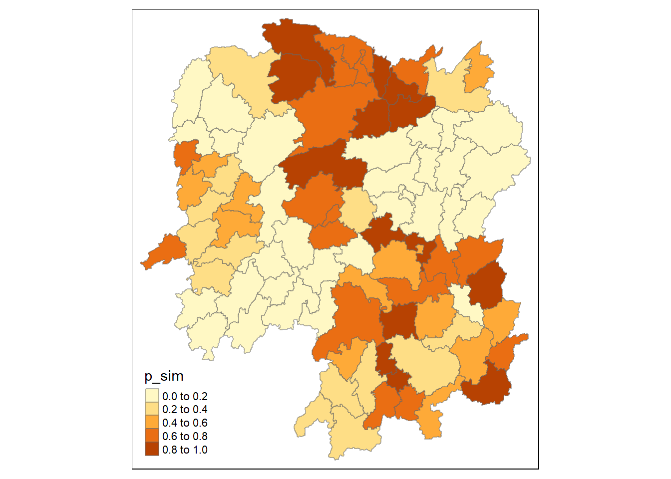
Emerging Hot Spots
GDPPC_date <- read_csv('data/aspatial/Hunan_GDPPC.csv')Create Time Series Cube
GDPPC_st <- spacetime(GDPPC_date, hunan, .loc_col = "County", .time_col = "Year")is_spacetime_cube(GDPPC_st)[1] TRUEGDPPC_nb <- GDPPC_st %>%
activate("geometry") %>%
mutate(
nb = include_self(st_contiguity(geometry)),
wt = st_inverse_distance(nb, geometry,
scale = 1,
alpha = 1)
) %>%
set_nbs("nb") %>%
set_wts("wt")Computing Gi*
gi_stars <- GDPPC_nb %>%
  group_by(Year) %>%
  mutate(gi_star = local_gstar_perm(GDPPC, nb, wt, nsim=99),
         .before = 1) %>%
  unnest(gi_star)
Mann-Kendall Test
cbg <- gi_stars %>%
  ungroup() %>%
  filter(County == "Changsha") %>%
  select(County, Year, gi_star)
ehsa <- emerging_hotspot_analysis(
GDPPC_st,
.var = "GDPPC",
k = 1,
nsim = 99
)ggplot(data = cbg,
aes(x = Year,
y = gi_star)) +
geom_line() +
theme_light()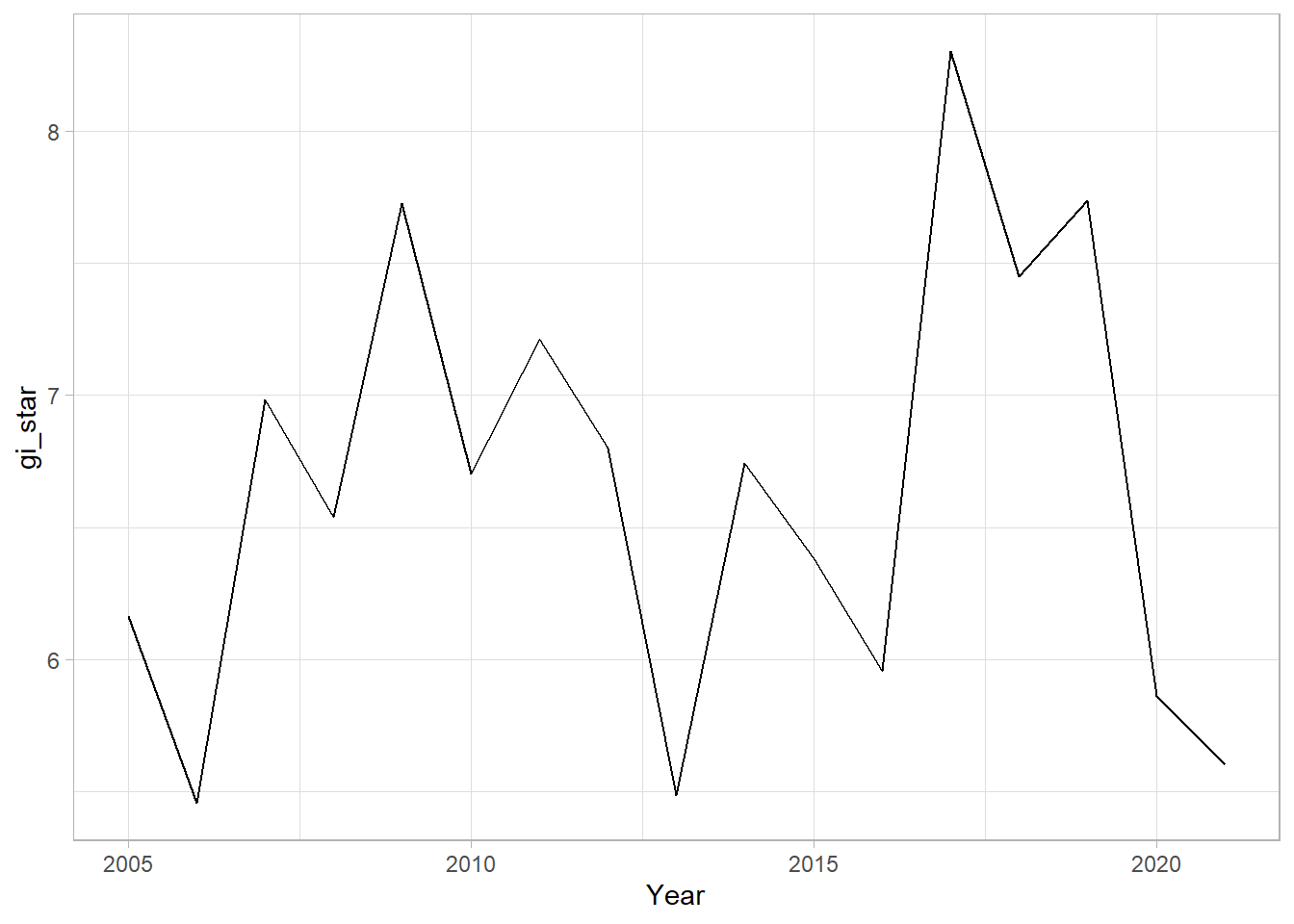
p <- ggplot(data = cbg,
       aes(x = Year,
           y = gi_star)) +
  geom_line() +
  theme_light()

ggplotly(p)
cbg %>%
summarise(mk = list(
unclass(
Kendall::MannKendall(gi_star)))) %>%
tidyr::unnest_wider(mk)# A tibble: 1 × 5
tau sl S D varS
<dbl> <dbl> <dbl> <dbl> <dbl>
1 0.0441 0.837 6 136. 589.Do for all locations
ehsa <- gi_stars %>%
  group_by(County) %>%
  summarise(mk = list(
    unclass(
      Kendall::MannKendall(gi_star)))) %>%
  tidyr::unnest_wider(mk)
Arrange to show significant emerging hot spots
emerging <- ehsa %>%
  arrange(sl, abs(tau)) %>%
  slice(1:5)
Perform EHSA with sfdep
ehsa <- emerging_hotspot_analysis(
  x = GDPPC_st,
  .var = "GDPPC",
  k = 1,
  nsim = 99
)ggplot(data = ehsa,
aes(x = classification)) +
geom_bar()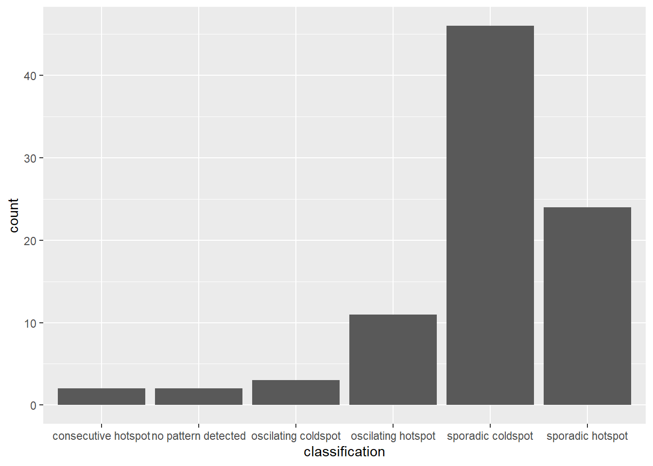
hunan_ehsa <- hunan %>%
left_join(ehsa,
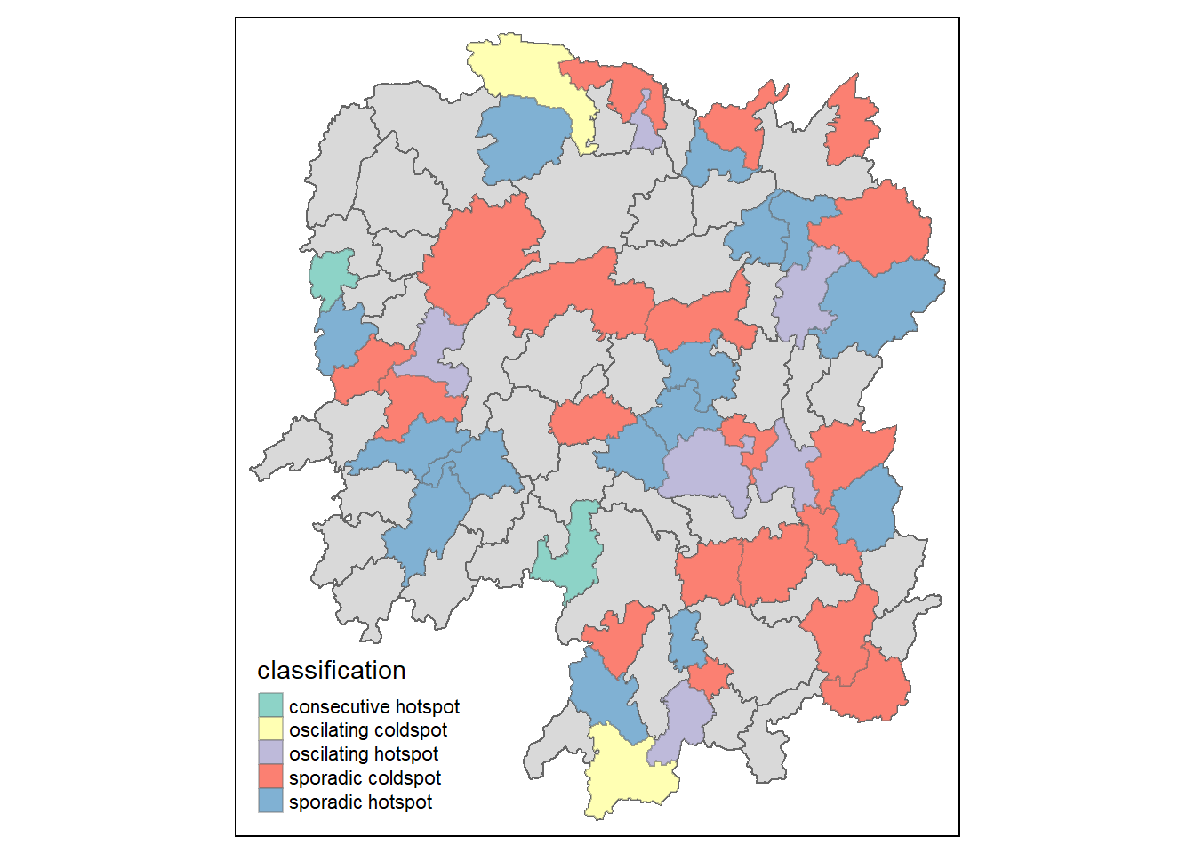
by = c("County" = "location"))ehsa_sig <- hunan_ehsa %>%
filter(p_value < 0.05)
tmap_mode("plot")
tm_shape(hunan_ehsa) +
tm_polygons() +
tm_borders(alpha = 0.5) +
tm_shape(ehsa_sig) +
tm_fill("classification") +
tm_borders(alpha = 0.4)