pacman::p_load(tmap, SpatialAcc, sf,
               ggstatsplot, reshape2,
tidyverse)In-Class Exercise 10: Modelling Geographical Accessibility
Import Packages
Import Data
Geospatial
mpsz <- st_read(dsn = "data/geospatial", layer = "MP14_SUBZONE_NO_SEA_PL")Reading layer `MP14_SUBZONE_NO_SEA_PL' from data source
`C:\Jenpoer\IS415-GAA\In-Class-Exercises\chapter-16\data\geospatial'
using driver `ESRI Shapefile'
Simple feature collection with 323 features and 15 fields
Geometry type: MULTIPOLYGON
Dimension: XY
Bounding box: xmin: 2667.538 ymin: 15748.72 xmax: 56396.44 ymax: 50256.33
Projected CRS: SVY21hexagons <- st_read(dsn = "data/geospatial", layer = "hexagons") Reading layer `hexagons' from data source
`C:\Jenpoer\IS415-GAA\In-Class-Exercises\chapter-16\data\geospatial'
using driver `ESRI Shapefile'
Simple feature collection with 3125 features and 6 fields
Geometry type: POLYGON
Dimension: XY
Bounding box: xmin: 2667.538 ymin: 21506.33 xmax: 50010.26 ymax: 50256.33
Projected CRS: SVY21 / Singapore TMeldercare <- st_read(dsn = "data/geospatial", layer = "ELDERCARE")Reading layer `ELDERCARE' from data source
`C:\Jenpoer\IS415-GAA\In-Class-Exercises\chapter-16\data\geospatial'
using driver `ESRI Shapefile'
Simple feature collection with 120 features and 19 fields
Geometry type: POINT
Dimension: XY
Bounding box: xmin: 14481.92 ymin: 28218.43 xmax: 41665.14 ymax: 46804.9
Projected CRS: SVY21 / Singapore TMAspatial
ODMatrix <- read_csv("data/aspatial/OD_Matrix.csv", skip = 0)Data Preprocessing
Update CRS
mpsz <- st_transform(mpsz, 3414)
eldercare <- st_transform(eldercare, 3414)
hexagons <- st_transform(hexagons, 3414)
Select relevant columns
We select only the relevant columns for the analysis. In addition, we create dummy columns for capacity (eldercare) and demand (hexagons). In reality, we actually have to look through the data (e.g. visit the eldercare websites) to know their actual demand.
eldercare <- eldercare %>%
  select(fid, ADDRESSPOS) %>%
  rename(destination_id = fid,
         postal_code = ADDRESSPOS) %>%
  mutate(capacity = 100)
hexagons <- hexagons %>%
select(fid) %>%
rename(origin_id = fid) %>%
mutate(demand = 100)Tidying aspatial data
We have the ODMatrix from aspatial data. All we need to do is to convert it into a matrix format.
distmat <- ODMatrix %>%
  select(origin_id, destination_id, total_cost) %>%
  pivot_wider(names_from="destination_id", values_from="total_cost")%>%
  select(c(-c('origin_id')))
Convert into kilometres
distmat_km <- as.matrix(distmat/1000)What if you don’t have the OD matrix?
We can calculate a continuous distance matrix with Euclidean distance.
1) Extract the coordinates
eldercare_coord <- st_coordinates(eldercare)
hexagons_coord <- st_coordinates(hexagons)
2) Calculate Euclidean matrix
EucMatrix <- SpatialAcc::distance(hexagons_coord,
                                  eldercare_coord, type="euclidean")
Modelling Accessibility
Hansen’s Method
acc_Hansen <- data.frame(ac(hexagons$demand,
                            eldercare$capacity,
                            distmat_km,
                            #d0 = 50,
                            power = 2,
                            family = "Hansen"))


colnames(acc_Hansen) <- "accHansen"

acc_Hansen <- as_tibble(acc_Hansen)

hexagon_Hansen <- bind_cols(hexagons, acc_Hansen)head(hexagon_Hansen)Simple feature collection with 6 features and 3 fields
Geometry type: POLYGON
Dimension: XY
Bounding box: xmin: 2667.538 ymin: 22756.33 xmax: 3244.888 ymax: 27756.33
Projected CRS: SVY21 / Singapore TM
origin_id demand accHansen geometry
1 1 100 1.648313e-14 POLYGON ((2667.538 27506.33...
2 2 100 1.096143e-16 POLYGON ((2667.538 25006.33...
3 3 100 3.865857e-17 POLYGON ((2667.538 24506.33...
4 4 100 1.482856e-17 POLYGON ((2667.538 24006.33...
5 5 100 1.051348e-17 POLYGON ((2667.538 23506.33...
6 6 100 5.076391e-18 POLYGON ((2667.538 23006.33...Visualisation
mapex <- st_bbox(hexagons)tmap_mode("plot")
tm_shape(hexagon_Hansen,
bbox = mapex) +
tm_fill(col = "accHansen",
n = 10,
style = "quantile",
border.col = "black",
border.lwd = 1) +
tm_shape(eldercare) +
tm_symbols(size = 0.1) +
tm_layout(main.title = "Accessibility to eldercare: Hansen method",
main.title.position = "center",
main.title.size = 2,
legend.outside = F,
legend.height = 0.45,
legend.width = 0.5,
legend.format = list(digits = 6),
legend.position = c("right", "top"),
frame = TRUE) +
tm_compass(type="8star", size = 2) +
tm_scale_bar(width = 0.15) +
tm_grid(lwd = 0.1, alpha = 0.5)
Boxplot summarized by region:
hexagon_Hansen <- st_join(hexagon_Hansen, mpsz,
join = st_intersects)ggplot(data=hexagon_Hansen,
aes(y = log(accHansen),
x= REGION_N)) +
geom_boxplot() +
geom_point(stat="summary",
fun.y="mean",
colour ="red",
size=2)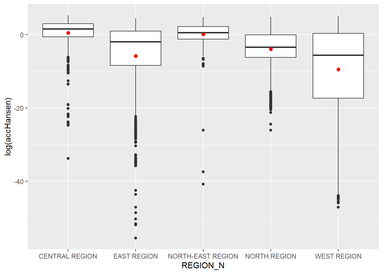
KD2SFCA Method
acc_KD2SFCA <- data.frame(ac(hexagons$demand,
                            eldercare$capacity,
                            distmat_km,
                            d0 = 50,
                            power = 2,
                            family = "KD2SFCA"))

colnames(acc_KD2SFCA) <- "accKD2SFCA"
acc_KD2SFCA <- as_tibble(acc_KD2SFCA)
hexagon_KD2SFCA <- bind_cols(hexagons, acc_KD2SFCA)
Visualisation
tmap_mode("plot")
tm_shape(hexagon_KD2SFCA,
         bbox = mapex) +
  tm_fill(col = "accKD2SFCA",
          n = 10,
          style = "quantile",
          border.col = "black",
          border.lwd = 1) +
tm_shape(eldercare) +
  tm_symbols(size = 0.1) +
  tm_layout(main.title = "Accessibility to eldercare: KD2SFCA method",
            main.title.position = "center",
            main.title.size = 2,
            legend.outside = FALSE,
            legend.height = 0.45,
            legend.width = 3.0,
            legend.format = list(digits = 6),
            legend.position = c("right", "top"),
            frame = TRUE) +
  tm_compass(type="8star", size = 2) +
  tm_scale_bar(width = 0.15) +
  tm_grid(lwd = 0.1, alpha = 0.5)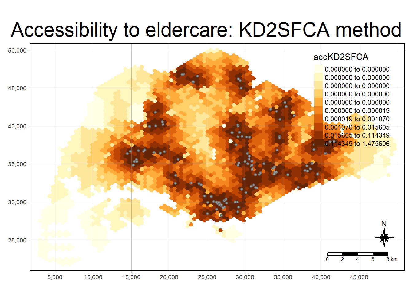
Boxplot summarized by region:
hexagon_KD2SFCA <- st_join(hexagon_KD2SFCA, mpsz,
join = st_intersects)ggplot(data=hexagon_KD2SFCA,
aes(y = accKD2SFCA,
x= REGION_N)) +
geom_boxplot() +
geom_point(stat="summary",
fun.y="mean",
colour ="red",
size=2)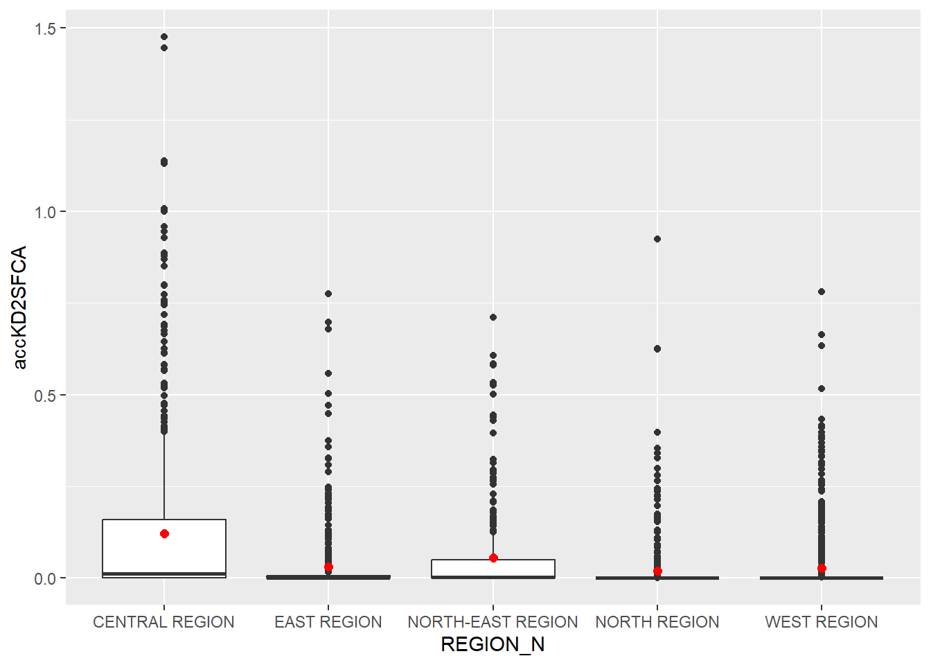
SAM Accessibility
acc_SAM <- data.frame(ac(hexagons$demand,
                         eldercare$capacity,
                         distmat_km,
                         d0 = 50,
                         power = 2,
                         family = "SAM"))

colnames(acc_SAM) <- "accSAM"
acc_SAM <- as_tibble(acc_SAM)
hexagon_SAM <- bind_cols(hexagons, acc_SAM)
Visualisation
tmap_mode("plot")
tm_shape(hexagon_SAM,
         bbox = mapex) +
  tm_fill(col = "accSAM",
          n = 10,
          style = "quantile",
          border.col = "black",
          border.lwd = 1) +
tm_shape(eldercare) +
  tm_symbols(size = 0.1) +
  tm_layout(main.title = "Accessibility to eldercare: SAM method",
            main.title.position = "center",
            main.title.size = 2,
            legend.outside = FALSE,
            legend.height = 0.45,
            legend.width = 3.0,
            legend.format = list(digits = 3),
            legend.position = c("right", "top"),
            frame = TRUE) +
  tm_compass(type="8star", size = 2) +
  tm_scale_bar(width = 0.15) +
  tm_grid(lwd = 0.1, alpha = 0.5)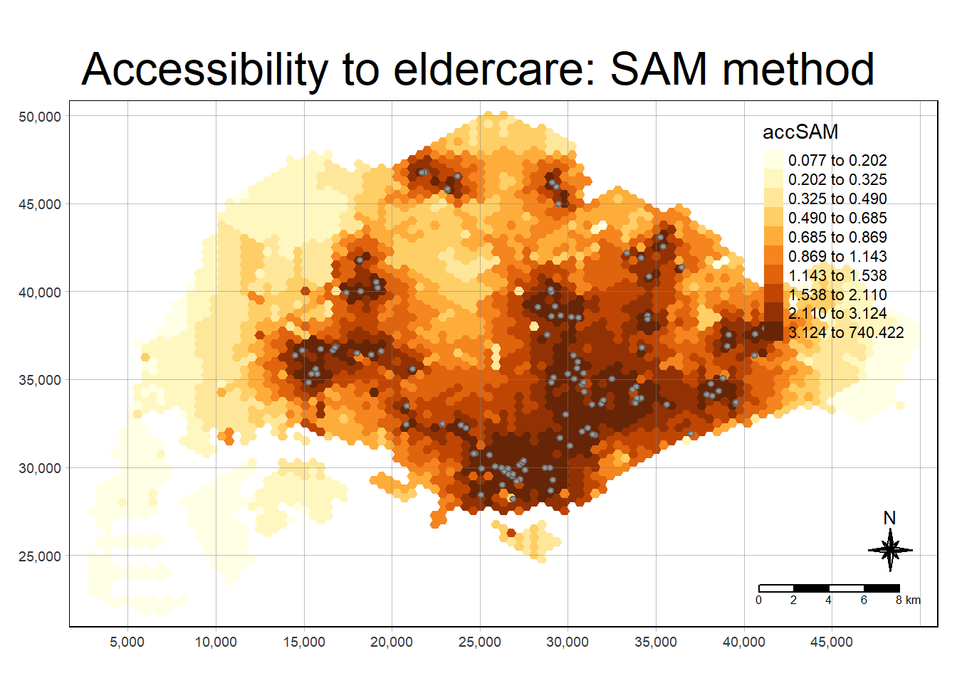
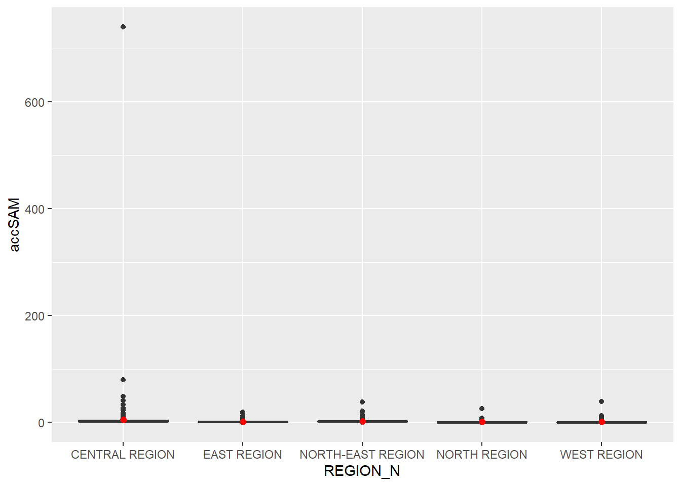
Box plot summarized by region:
hexagon_SAM <- st_join(hexagon_SAM, mpsz,
join = st_intersects)ggplot(data=hexagon_SAM,
aes(y = accSAM,
x= REGION_N)) +
geom_boxplot() +
geom_point(stat="summary",
fun.y="mean",
colour ="red",
size=2)