In-Class Exercise 6: Spatial Weights and Applications

Import Packages

pacman::p_load(sf, sfdep, tmap, tidyverse)

Import Dataset

Geospatial

hunan <- st_read(dsn = "data/geospatial", 
                 layer = "Hunan")

Reading layer `Hunan' from data source 
  `C:\Jenpoer\IS415-GAA\In-Class-Exercises\chapter-06\data\geospatial' 
  using driver `ESRI Shapefile'
Simple feature collection with 88 features and 7 fields
Geometry type: POLYGON
Dimension:     XY
Bounding box:  xmin: 108.7831 ymin: 24.6342 xmax: 114.2544 ymax: 30.12812
Geodetic CRS:  WGS 84

Aspatial

hunan2012 <- read_csv("data/aspatial/Hunan_2012.csv")

Data Preprocessing

Combining data frame with left join

If you want to retain geometry, the left one must be the geospatial data

hunan_GDPPC <- left_join(hunan,hunan2012) %>%
  select(1:4, 7, 15)

tm_shape(hunan_GDPPC)+
  tm_fill("GDPPC", 
          style = "quantile", 
          palette = "Blues",
          title = "GDPPC") +
  tm_layout(main.title = "Distribution of GDP per capita by district, Hunan Province",
            main.title.position = "center",
            main.title.size = 1,
            legend.outside = TRUE,
            legend.position = c("right", "bottom"),
            frame = TRUE) +
  tm_borders(alpha=0.5) +
  tm_compass(type="8star", size = 2) +
  tm_scale_bar() +
  tm_grid(alpha = 0.2)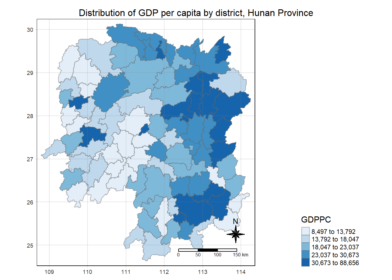

Identify Polygon Neighbors

wm_q <- hunan_GDPPC %>%
  mutate(nb = st_contiguity(geometry),
         wt = st_weights(nb),
         .before = 1) # put newly-created field in first column

wm_r <- hunan_GDPPC %>%
  mutate(nb = st_contiguity(geometry, queen = TRUE),
         wt = st_weights(nb),
         .before = 1) # put newly-created field in first column