pacman::p_load(sf, tidyverse)Hands-On Exercise 2: Geospatial Data Wrangling
Import Packages
Spatial Data
Importing the Datasets
Master Plan 2014 Subzone Boundaries (Web) from data.gov.sg . Web version is used because it’s optimized for web display, with a smaller file size.
mpsz = st_read(dsn = "data/geospatial/master-plan-2014-subzone-boundary-web-shp",
               layer = "MP14_SUBZONE_WEB_PL")
Reading layer `MP14_SUBZONE_WEB_PL' from data source
`C:\Jenpoer\IS415-GAA\Hands-On-Exercises\chapter-02\data\geospatial\master-plan-2014-subzone-boundary-web-shp'
using driver `ESRI Shapefile'
Simple feature collection with 323 features and 15 fields
Geometry type: MULTIPOLYGON
Dimension: XY
Bounding box: xmin: 2667.538 ymin: 15748.72 xmax: 56396.44 ymax: 50256.33
Projected CRS: SVY21Cycling Path from LTADataMall
cyclingpath = st_read(dsn = "data/geospatial/CyclingPathGazette",
                      layer = "CyclingPathGazette")
Reading layer `CyclingPathGazette' from data source
`C:\Jenpoer\IS415-GAA\Hands-On-Exercises\chapter-02\data\geospatial\CyclingPathGazette'
using driver `ESRI Shapefile'
Simple feature collection with 2248 features and 2 fields
Geometry type: MULTILINESTRING
Dimension: XY
Bounding box: xmin: 11854.32 ymin: 28347.98 xmax: 42626.09 ymax: 48948.15
Projected CRS: SVY21Pre-Schools Location from Dataportal.asia (originally from data.gov.sg)
preschool = st_read("data/geospatial/preschools-location.kml")Reading layer `PRESCHOOLS_LOCATION' from data source
`C:\Jenpoer\IS415-GAA\Hands-On-Exercises\chapter-02\data\geospatial\preschools-location.kml'
using driver `KML'
Simple feature collection with 1925 features and 2 fields
Geometry type: POINT
Dimension: XYZ
Bounding box: xmin: 103.6824 ymin: 1.247759 xmax: 103.9897 ymax: 1.462134
z_range: zmin: 0 zmax: 0
Geodetic CRS: WGS 84Checking the contents of a simple feature data frame
Checking the information about the geometry, such as type, geographic extent of features, and coordinate system of the data.
st_geometry(mpsz)Geometry set for 323 features
Geometry type: MULTIPOLYGON
Dimension: XY
Bounding box: xmin: 2667.538 ymin: 15748.72 xmax: 56396.44 ymax: 50256.33
Projected CRS: SVY21
First 5 geometries:Find out about the attribute information in the data frame.
glimpse(mpsz)Rows: 323
Columns: 16
$ OBJECTID <int> 1, 2, 3, 4, 5, 6, 7, 8, 9, 10, 11, 12, 13, 14, 15, 16, 17, …
$ SUBZONE_NO <int> 1, 1, 3, 8, 3, 7, 9, 2, 13, 7, 12, 6, 1, 5, 1, 1, 3, 2, 2, …
$ SUBZONE_N <chr> "MARINA SOUTH", "PEARL'S HILL", "BOAT QUAY", "HENDERSON HIL…
$ SUBZONE_C <chr> "MSSZ01", "OTSZ01", "SRSZ03", "BMSZ08", "BMSZ03", "BMSZ07",…
$ CA_IND <chr> "Y", "Y", "Y", "N", "N", "N", "N", "Y", "N", "N", "N", "N",…
$ PLN_AREA_N <chr> "MARINA SOUTH", "OUTRAM", "SINGAPORE RIVER", "BUKIT MERAH",…
$ PLN_AREA_C <chr> "MS", "OT", "SR", "BM", "BM", "BM", "BM", "SR", "QT", "QT",…
$ REGION_N <chr> "CENTRAL REGION", "CENTRAL REGION", "CENTRAL REGION", "CENT…
$ REGION_C <chr> "CR", "CR", "CR", "CR", "CR", "CR", "CR", "CR", "CR", "CR",…
$ INC_CRC <chr> "5ED7EB253F99252E", "8C7149B9EB32EEFC", "C35FEFF02B13E0E5",…
$ FMEL_UPD_D <date> 2014-12-05, 2014-12-05, 2014-12-05, 2014-12-05, 2014-12-05…
$ X_ADDR <dbl> 31595.84, 28679.06, 29654.96, 26782.83, 26201.96, 25358.82,…
$ Y_ADDR <dbl> 29220.19, 29782.05, 29974.66, 29933.77, 30005.70, 29991.38,…
$ SHAPE_Leng <dbl> 5267.381, 3506.107, 1740.926, 3313.625, 2825.594, 4428.913,…
$ SHAPE_Area <dbl> 1630379.27, 559816.25, 160807.50, 595428.89, 387429.44, 103…
$ geometry <MULTIPOLYGON [m]> MULTIPOLYGON (((31495.56 30..., MULTIPOLYGON (…Reveal complete information of a feature object, but retrieve the first few rows only.
head(mpsz, n=5)Simple feature collection with 5 features and 15 fields
Geometry type: MULTIPOLYGON
Dimension: XY
Bounding box: xmin: 25867.68 ymin: 28369.47 xmax: 32362.39 ymax: 30435.54
Projected CRS: SVY21
OBJECTID SUBZONE_NO SUBZONE_N SUBZONE_C CA_IND PLN_AREA_N
1 1 1 MARINA SOUTH MSSZ01 Y MARINA SOUTH
2 2 1 PEARL'S HILL OTSZ01 Y OUTRAM
3 3 3 BOAT QUAY SRSZ03 Y SINGAPORE RIVER
4 4 8 HENDERSON HILL BMSZ08 N BUKIT MERAH
5 5 3 REDHILL BMSZ03 N BUKIT MERAH
PLN_AREA_C REGION_N REGION_C INC_CRC FMEL_UPD_D X_ADDR
1 MS CENTRAL REGION CR 5ED7EB253F99252E 2014-12-05 31595.84
2 OT CENTRAL REGION CR 8C7149B9EB32EEFC 2014-12-05 28679.06
3 SR CENTRAL REGION CR C35FEFF02B13E0E5 2014-12-05 29654.96
4 BM CENTRAL REGION CR 3775D82C5DDBEFBD 2014-12-05 26782.83
5 BM CENTRAL REGION CR 85D9ABEF0A40678F 2014-12-05 26201.96
Y_ADDR SHAPE_Leng SHAPE_Area geometry
1 29220.19 5267.381 1630379.3 MULTIPOLYGON (((31495.56 30...
2 29782.05 3506.107 559816.2 MULTIPOLYGON (((29092.28 30...
3 29974.66 1740.926 160807.5 MULTIPOLYGON (((29932.33 29...
4 29933.77 3313.625 595428.9 MULTIPOLYGON (((27131.28 30...
5 30005.70 2825.594 387429.4 MULTIPOLYGON (((26451.03 30...Plotting the Geospatial Data
Plot all the features of the data frame in small multiples. max.plot is used to show all the features, since it limits to the first 9 by default.
plot(mpsz, max.plot=15)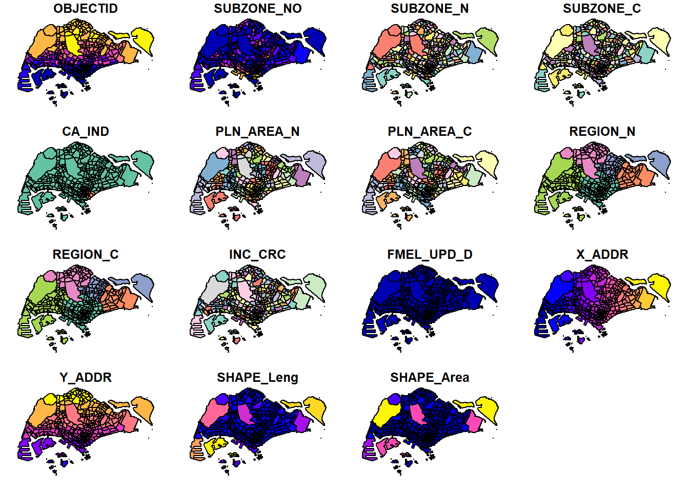
Plot only the geometry
plot(st_geometry(mpsz))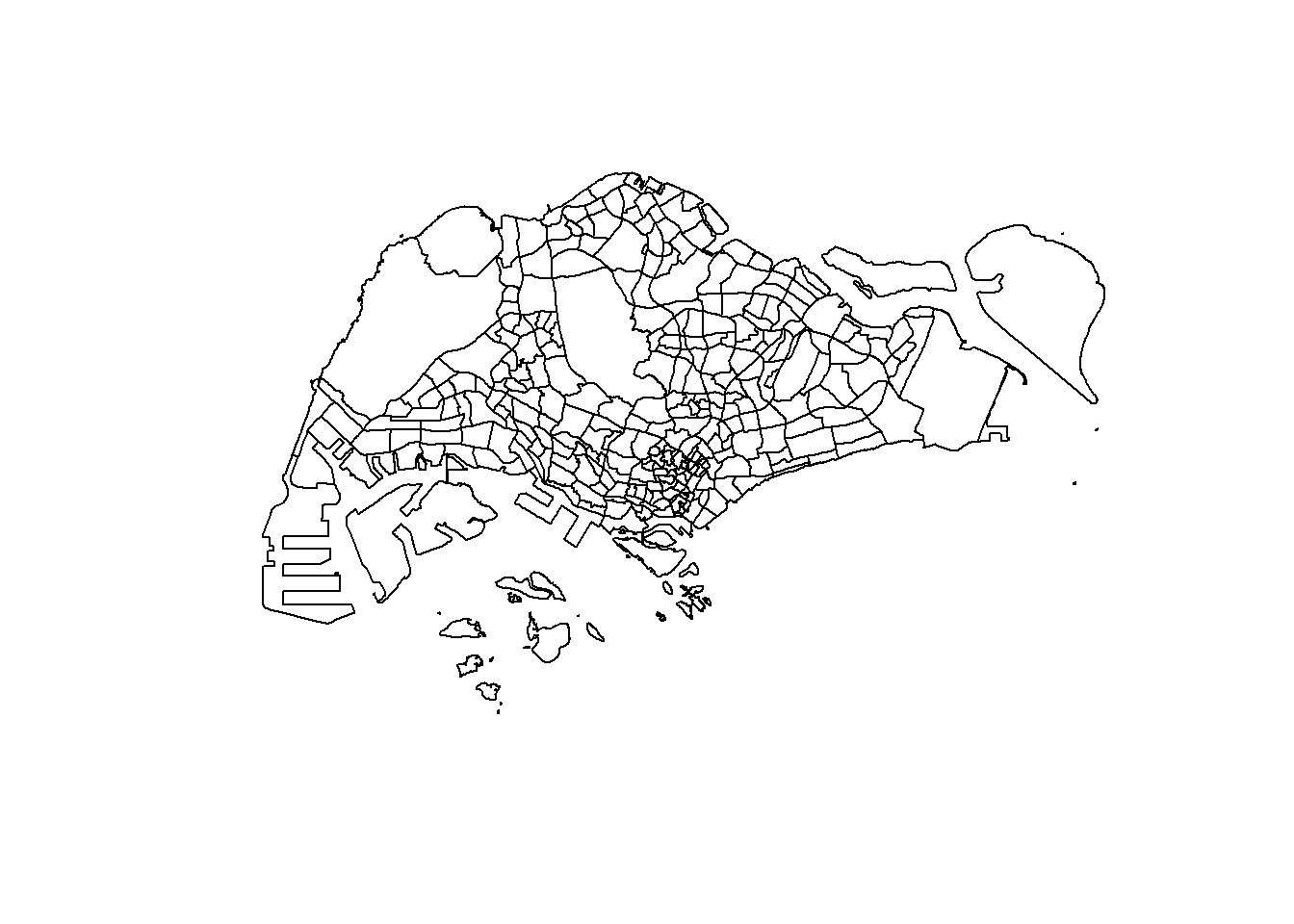
Plot the sf object using a specific attribute
plot(mpsz["PLN_AREA_N"])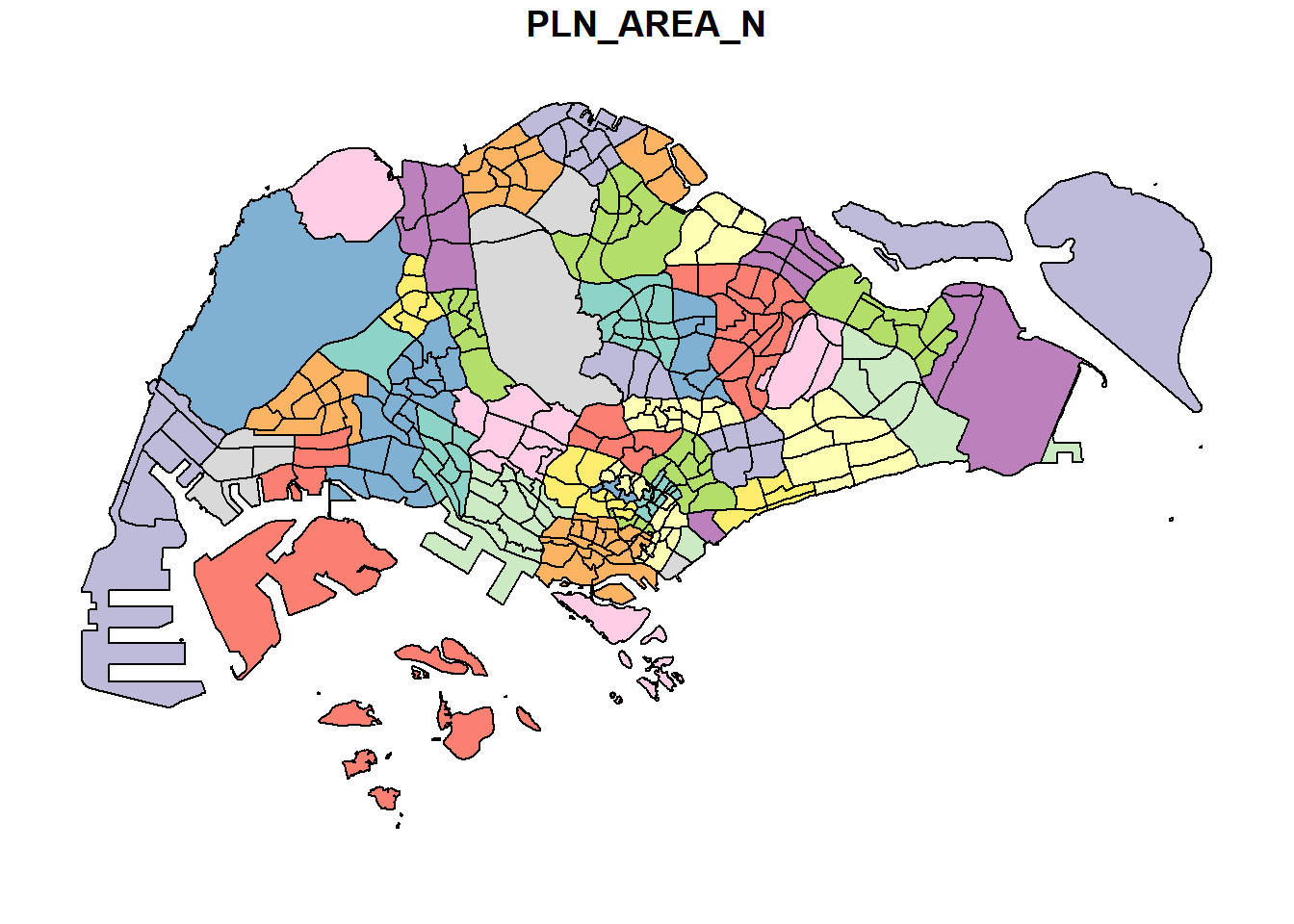
Projection Transformation
Project a feature to another coordinate system.
st_crs(mpsz)Coordinate Reference System:
User input: SVY21
wkt:
PROJCRS["SVY21",
BASEGEOGCRS["SVY21[WGS84]",
DATUM["World Geodetic System 1984",
ELLIPSOID["WGS 84",6378137,298.257223563,
LENGTHUNIT["metre",1]],
ID["EPSG",6326]],
PRIMEM["Greenwich",0,
ANGLEUNIT["Degree",0.0174532925199433]]],
CONVERSION["unnamed",
METHOD["Transverse Mercator",
ID["EPSG",9807]],
PARAMETER["Latitude of natural origin",1.36666666666667,
ANGLEUNIT["Degree",0.0174532925199433],
ID["EPSG",8801]],
PARAMETER["Longitude of natural origin",103.833333333333,
ANGLEUNIT["Degree",0.0174532925199433],
ID["EPSG",8802]],
PARAMETER["Scale factor at natural origin",1,
SCALEUNIT["unity",1],
ID["EPSG",8805]],
PARAMETER["False easting",28001.642,
LENGTHUNIT["metre",1],
ID["EPSG",8806]],
PARAMETER["False northing",38744.572,
LENGTHUNIT["metre",1],
ID["EPSG",8807]]],
CS[Cartesian,2],
AXIS["(E)",east,
ORDER[1],
LENGTHUNIT["metre",1,
ID["EPSG",9001]]],
AXIS["(N)",north,
ORDER[2],
LENGTHUNIT["metre",1,
ID["EPSG",9001]]]]Even though the projection system is SVY21, when we read the end of print, the EPSG is 9001. This is wrong because EPSG of SVY21 should be 3414.
SVY21 is coordinate system for Singapore.
mpsz3414 <- st_set_crs(mpsz, 3414)However, different case for Preschool. We cannot just replace the EPSG.
st_geometry(preschool)Geometry set for 1925 features
Geometry type: POINT
Dimension: XYZ
Bounding box: xmin: 103.6824 ymin: 1.247759 xmax: 103.9897 ymax: 1.462134
z_range: zmin: 0 zmax: 0
Geodetic CRS: WGS 84
First 5 geometries:It uses WGS84, which we need to actually project mathematically to SVY21.
preschool3414 <- st_transform(preschool,
                              crs = 3414)
Aspatial Data
Import data
listings <- read_csv('data/aspatial/listings.csv')
list(listings)
[[1]]
# A tibble: 4,161 × 18
id name host_id host_…¹ neigh…² neigh…³ latit…⁴ longi…⁵ room_…⁶ price
<dbl> <chr> <dbl> <chr> <chr> <chr> <dbl> <dbl> <chr> <dbl>
1 50646 Pleasan… 227796 Sujatha Centra… Bukit … 1.33 104. Privat… 80
2 71609 Ensuite… 367042 Belinda East R… Tampin… 1.35 104. Privat… 145
3 71896 B&B Ro… 367042 Belinda East R… Tampin… 1.35 104. Privat… 85
4 71903 Room 2-… 367042 Belinda East R… Tampin… 1.35 104. Privat… 85
5 275344 15 mins… 1439258 Kay Centra… Bukit … 1.29 104. Privat… 49
6 289234 Booking… 367042 Belinda East R… Tampin… 1.34 104. Privat… 184
7 294281 5 mins … 1521514 Elizab… Centra… Newton 1.31 104. Privat… 79
8 324945 Cozy Bl… 1439258 Kay Centra… Bukit … 1.29 104. Privat… 49
9 330089 Cozy Bl… 1439258 Kay Centra… Bukit … 1.29 104. Privat… 55
10 330095 10 mins… 1439258 Kay Centra… Bukit … 1.29 104. Privat… 55
# … with 4,151 more rows, 8 more variables: minimum_nights <dbl>,
# number_of_reviews <dbl>, last_review <date>, reviews_per_month <dbl>,
# calculated_host_listings_count <dbl>, availability_365 <dbl>,
# number_of_reviews_ltm <dbl>, license <chr>, and abbreviated variable names
# ¹host_name, ²neighbourhood_group, ³neighbourhood, ⁴latitude, ⁵longitude,
# ⁶room_typeListings is a tibble
is_tibble(listings)[1] TRUECreate a simple feature data frame from aspatial data
listings_sf <- st_as_sf(listings,
                        coords = c("longitude", "latitude"),
                        crs=4326) %>%
  st_transform(crs = 3414)
%>% is like a pipe, defined by package magrittr, used to pass the left hand side of the operator to the first argument of the right hand side of the operator
glimpse(listings_sf)Rows: 4,161
Columns: 17
$ id <dbl> 50646, 71609, 71896, 71903, 275344, 289…
$ name <chr> "Pleasant Room along Bukit Timah", "Ens…
$ host_id <dbl> 227796, 367042, 367042, 367042, 1439258…
$ host_name <chr> "Sujatha", "Belinda", "Belinda", "Belin…
$ neighbourhood_group <chr> "Central Region", "East Region", "East …
$ neighbourhood <chr> "Bukit Timah", "Tampines", "Tampines", …
$ room_type <chr> "Private room", "Private room", "Privat…
$ price <dbl> 80, 145, 85, 85, 49, 184, 79, 49, 55, 5…
$ minimum_nights <dbl> 92, 92, 92, 92, 60, 92, 92, 60, 60, 60,…
$ number_of_reviews <dbl> 18, 20, 24, 47, 14, 12, 133, 17, 12, 3,…
$ last_review <date> 2014-12-26, 2020-01-17, 2019-10-13, 20…
$ reviews_per_month <dbl> 0.18, 0.15, 0.18, 0.34, 0.11, 0.10, 1.0…
$ calculated_host_listings_count <dbl> 1, 6, 6, 6, 44, 6, 7, 44, 44, 44, 6, 7,…
$ availability_365 <dbl> 365, 340, 265, 365, 296, 285, 365, 181,…
$ number_of_reviews_ltm <dbl> 0, 0, 0, 0, 1, 0, 0, 3, 2, 0, 1, 0, 0, …
$ license <chr> NA, NA, NA, NA, "S0399", NA, NA, "S0399…
$ geometry <POINT [m]> POINT (22646.02 35167.9), POINT (…Geoprocessing
Buffering
Buffering is reclassification based on distance: classification of within/without a given proximity.
buffer_cycling <- st_buffer(cyclingpath,
                            dist=5, nQuadSegs = 30) # 5 meter buffers along cycling paths
Calculate area of buffers
buffer_cycling$AREA <- st_area(buffer_cycling)Show sum of total land involved
sum(buffer_cycling$AREA)1556978 [m^2]Point-in-polygon Count
Goal: Identify pre-schools located in each Planning Subzone using st_intersects.
length is used to calculate number of pre-schools that fall inside each zone.
mpsz3414$`PreSch Count`<- lengths(st_intersects(mpsz3414, listings_sf))summary(mpsz3414$`PreSch Count`) Min. 1st Qu. Median Mean 3rd Qu. Max.
0.000 0.000 2.000 9.709 8.000 253.000 List the subzone with the most number of preschools
top_n(mpsz3414, 1, `PreSch Count`)Simple feature collection with 1 feature and 16 fields
Geometry type: MULTIPOLYGON
Dimension: XY
Bounding box: xmin: 30342.65 ymin: 32035.6 xmax: 31453.96 ymax: 33233.11
Projected CRS: SVY21 / Singapore TM
OBJECTID SUBZONE_NO SUBZONE_N SUBZONE_C CA_IND PLN_AREA_N PLN_AREA_C
1 126 6 LAVENDER KLSZ06 N KALLANG KL
REGION_N REGION_C INC_CRC FMEL_UPD_D X_ADDR Y_ADDR
1 CENTRAL REGION CR A7A07F328A38B6EF 2014-12-05 30874.41 32569.53
SHAPE_Leng SHAPE_Area geometry PreSch Count
1 3609.15 757907.6 MULTIPOLYGON (((31389.56 32... 253Display count of preschools in subzone number
aggregate(`PreSch Count` ~ SUBZONE_NO, mpsz3414, FUN=sum) SUBZONE_NO PreSch Count
1 1 426
2 2 372
3 3 522
4 4 340
5 5 314
6 6 337
7 7 124
8 8 101
9 9 146
10 10 154
11 11 91
12 12 55
13 13 57
14 14 35
15 15 16
16 16 39
17 17 7Count density by planning subzone
mpsz3414$Area <- mpsz3414 %>%
  st_area()
mpsz3414 <- mpsz3414 %>%
  mutate(`PreSch Density` = `PreSch Count`/Area * 1000000)
head(mpsz3414)
Simple feature collection with 6 features and 18 fields
Geometry type: MULTIPOLYGON
Dimension: XY
Bounding box: xmin: 24468.89 ymin: 28369.47 xmax: 32362.39 ymax: 30542.74
Projected CRS: SVY21 / Singapore TM
OBJECTID SUBZONE_NO SUBZONE_N SUBZONE_C CA_IND PLN_AREA_N
1 1 1 MARINA SOUTH MSSZ01 Y MARINA SOUTH
2 2 1 PEARL'S HILL OTSZ01 Y OUTRAM
3 3 3 BOAT QUAY SRSZ03 Y SINGAPORE RIVER
4 4 8 HENDERSON HILL BMSZ08 N BUKIT MERAH
5 5 3 REDHILL BMSZ03 N BUKIT MERAH
6 6 7 ALEXANDRA HILL BMSZ07 N BUKIT MERAH
PLN_AREA_C REGION_N REGION_C INC_CRC FMEL_UPD_D X_ADDR
1 MS CENTRAL REGION CR 5ED7EB253F99252E 2014-12-05 31595.84
2 OT CENTRAL REGION CR 8C7149B9EB32EEFC 2014-12-05 28679.06
3 SR CENTRAL REGION CR C35FEFF02B13E0E5 2014-12-05 29654.96
4 BM CENTRAL REGION CR 3775D82C5DDBEFBD 2014-12-05 26782.83
5 BM CENTRAL REGION CR 85D9ABEF0A40678F 2014-12-05 26201.96
6 BM CENTRAL REGION CR 9D286521EF5E3B59 2014-12-05 25358.82
Y_ADDR SHAPE_Leng SHAPE_Area geometry PreSch Count
1 29220.19 5267.381 1630379.3 MULTIPOLYGON (((31495.56 30... 8
2 29782.05 3506.107 559816.2 MULTIPOLYGON (((29092.28 30... 26
3 29974.66 1740.926 160807.5 MULTIPOLYGON (((29932.33 29... 48
4 29933.77 3313.625 595428.9 MULTIPOLYGON (((27131.28 30... 2
5 30005.70 2825.594 387429.4 MULTIPOLYGON (((26451.03 30... 1
6 29991.38 4428.913 1030378.8 MULTIPOLYGON (((25899.7 297... 7
Area PreSch Density
1 1630379.3 [m^2] 4.906834 [1/m^2]
2 559816.2 [m^2] 46.443811 [1/m^2]
3 160807.5 [m^2] 298.493545 [1/m^2]
4 595428.9 [m^2] 3.358923 [1/m^2]
5 387429.4 [m^2] 2.581115 [1/m^2]
6 1030378.8 [m^2] 6.793618 [1/m^2]Exploratory Data Analysis (EDA)
Basic plot
hist(mpsz3414$`PreSch Density`)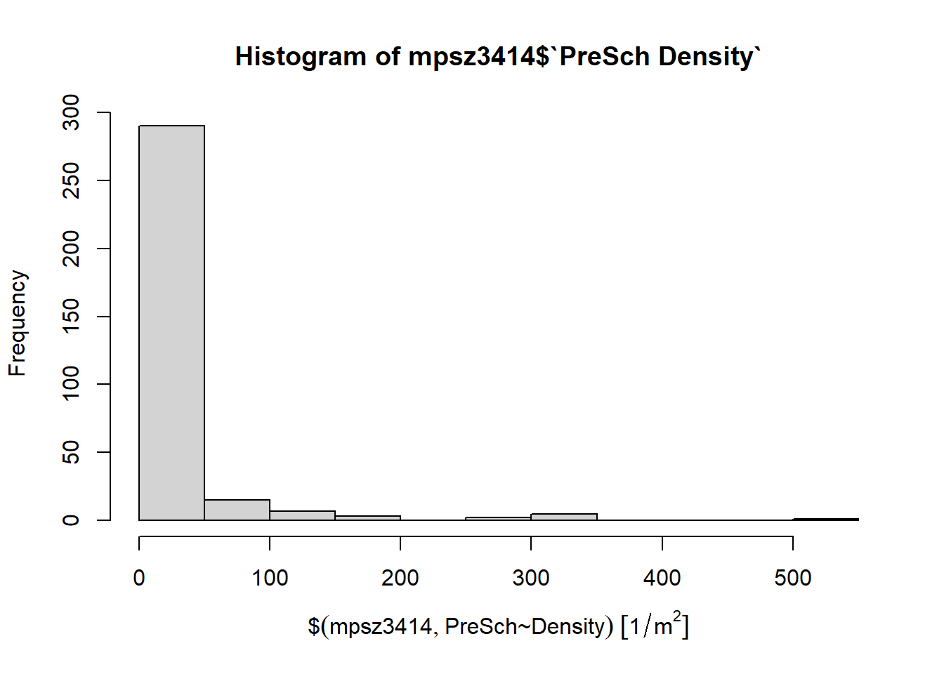
Fancier plot using ggplot2
ggplot(data=mpsz3414,
       aes(x= as.numeric(`PreSch Density`)))+
  geom_histogram(bins=20,
                 color="black",
                 fill="light blue") +
  labs(title = "Are pre-school even distributed in Singapore?",
       subtitle= "There are many planning sub-zones with a single pre-school, on the other hand, \nthere are two planning sub-zones with at least 20 pre-schools",
       x = "Pre-school density (per km sq)",
       y = "Frequency")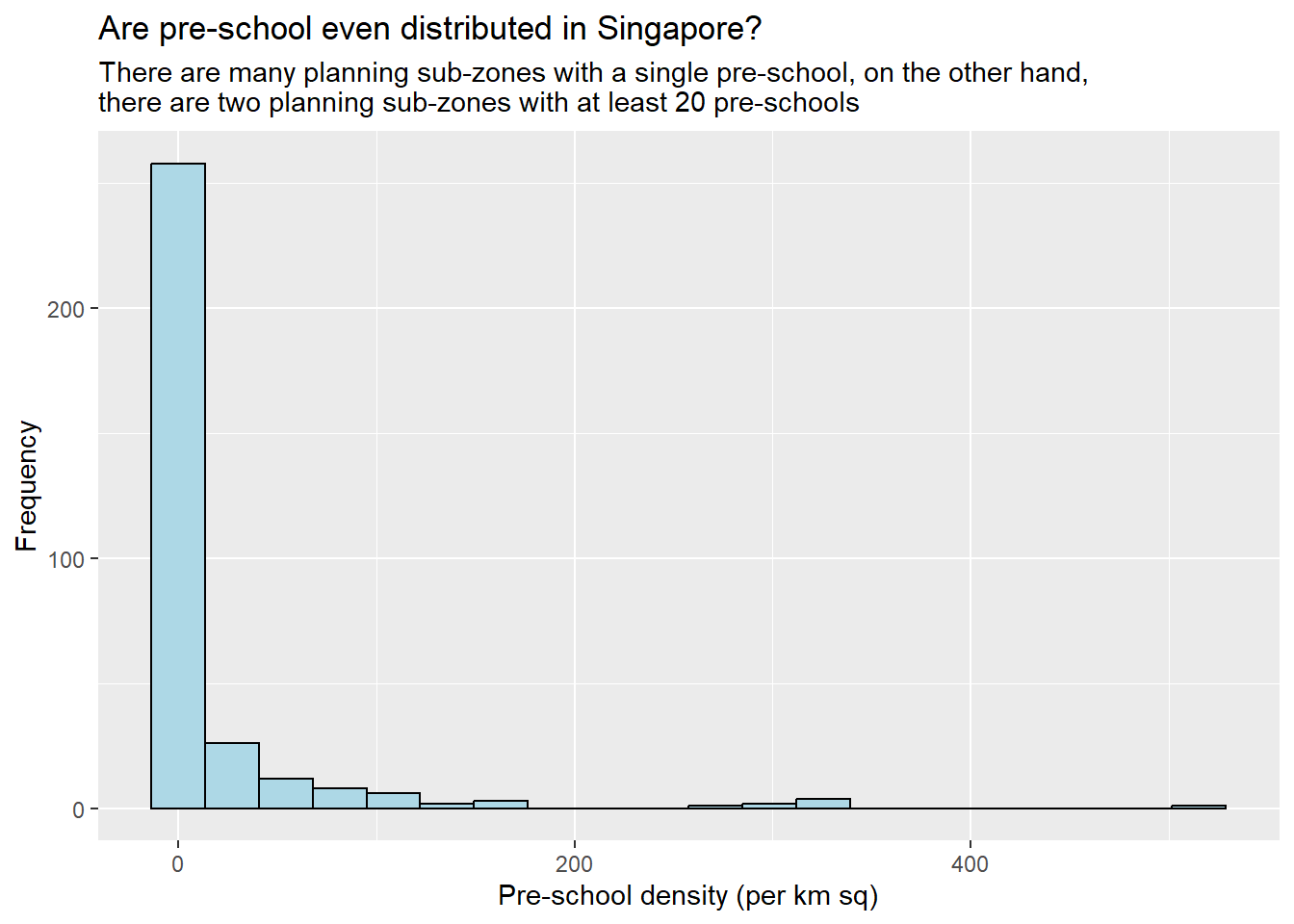
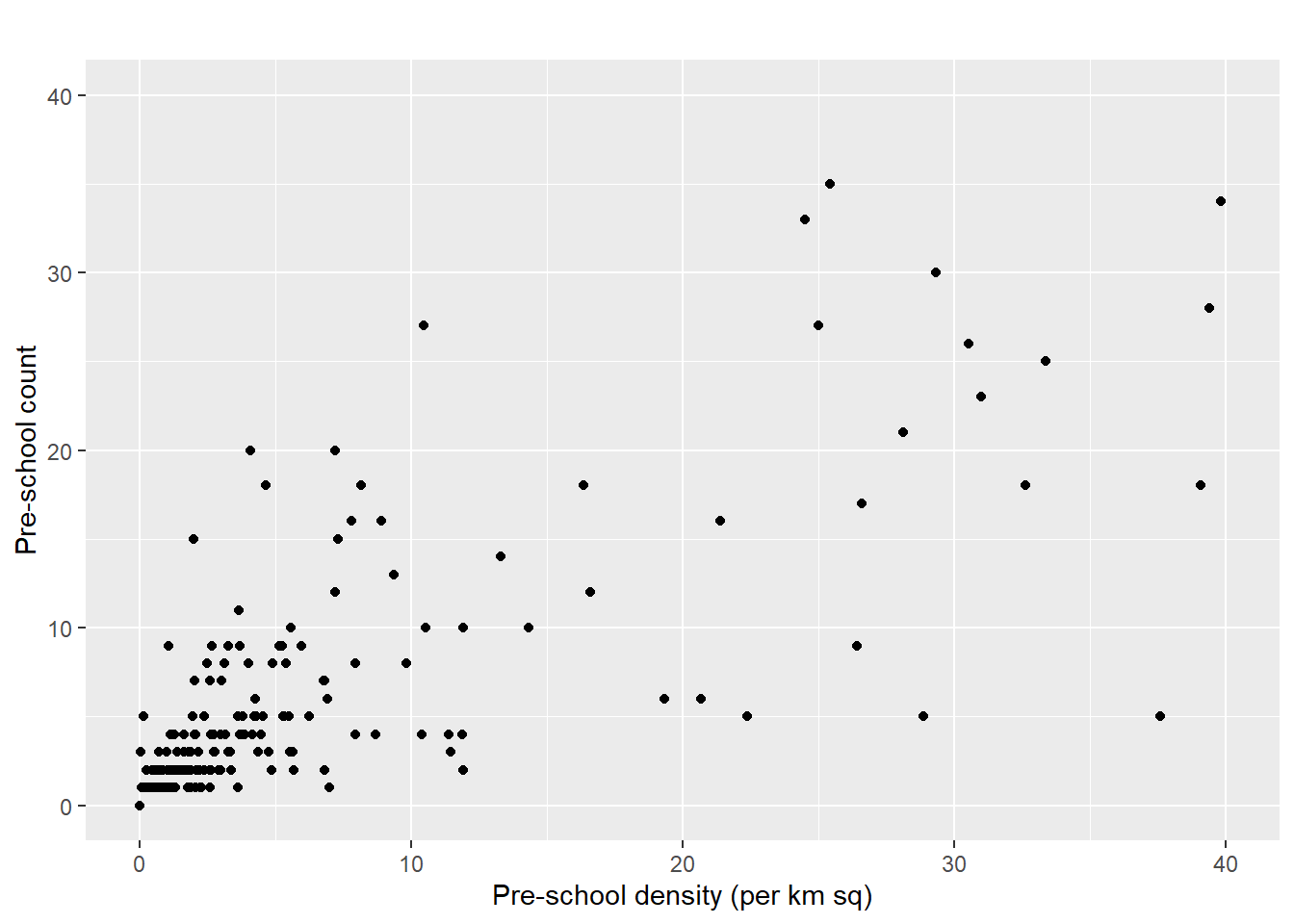
Scatter plot between preschool density and preschool count
ggplot(data=mpsz3414,
       aes(y = `PreSch Count`,
           x= as.numeric(`PreSch Density`)))+
  geom_point(color="black",
             fill="light blue") +
  xlim(0, 40) +
  ylim(0, 40) +
  labs(title = "",
       x = "Pre-school density (per km sq)",
       y = "Pre-school count")