In-Class Exercise 4: Spatial Points Patterns Analysis

Author

Jennifer Poernomo

Published

January 30, 2023

Modified

March 24, 2023

Importing packages

pacman::p_load(maptools, sf, raster, spatstat, tmap)

Importing data

Spatial data

childcare_sf <- st_read("../../Hands-On-Exercises/chapter-04/data/geospatial/childcare.geojson") %>%
  st_transform(crs = 3414)

Reading layer `childcare' from data source 
  `C:\Jenpoer\IS415-GAA\Hands-On-Exercises\chapter-04\data\geospatial\childcare.geojson' 
  using driver `GeoJSON'
Simple feature collection with 1545 features and 2 fields
Geometry type: POINT
Dimension:     XYZ
Bounding box:  xmin: 103.6824 ymin: 1.248403 xmax: 103.9897 ymax: 1.462134
z_range:       zmin: 0 zmax: 0
Geodetic CRS:  WGS 84

sg_sf <- st_read(dsn = "../../Hands-On-Exercises/chapter-04/data/geospatial/CostalOutline", layer="CostalOutline")

Reading layer `CostalOutline' from data source 
  `C:\Jenpoer\IS415-GAA\Hands-On-Exercises\chapter-04\data\geospatial\CostalOutline' 
  using driver `ESRI Shapefile'
Simple feature collection with 60 features and 4 fields
Geometry type: POLYGON
Dimension:     XY
Bounding box:  xmin: 2663.926 ymin: 16357.98 xmax: 56047.79 ymax: 50244.03
Projected CRS: SVY21

mpsz_sf <- st_read(dsn = "../../Hands-On-Exercises/chapter-02/data/geospatial/master-plan-2014-subzone-boundary-web-shp",
                   layer = "MP14_SUBZONE_WEB_PL")

Reading layer `MP14_SUBZONE_WEB_PL' from data source 
  `C:\Jenpoer\IS415-GAA\Hands-On-Exercises\chapter-02\data\geospatial\master-plan-2014-subzone-boundary-web-shp' 
  using driver `ESRI Shapefile'
Simple feature collection with 323 features and 15 fields
Geometry type: MULTIPOLYGON
Dimension:     XY
Bounding box:  xmin: 2667.538 ymin: 15748.72 xmax: 56396.44 ymax: 50256.33
Projected CRS: SVY21

Spatial*

childcare <- as_Spatial(childcare_sf)
mpsz <- as_Spatial(mpsz_sf)
sg <- as_Spatial(sg_sf)

sp object: Only retains the geometry

childcare_sp <- as(childcare, "SpatialPoints")
sg_sp <- as(sg, "SpatialPolygons")

ppp format

childcare_ppp <- as(childcare_sp, "ppp")
childcare_ppp

Planar point pattern: 1545 points
window: rectangle = [11203.01, 45404.24] x [25667.6, 49300.88] units

plot(childcare_ppp)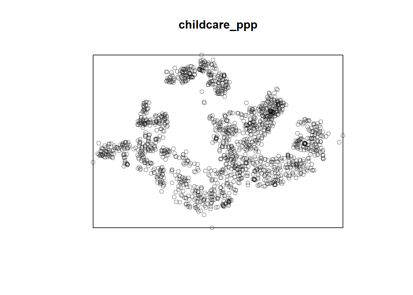

Create owin object

sg_owin <- as(sg_sp, "owin")

Combine with owin

childcareSG_ppp = childcare_ppp[sg_owin]
plot(childcareSG_ppp)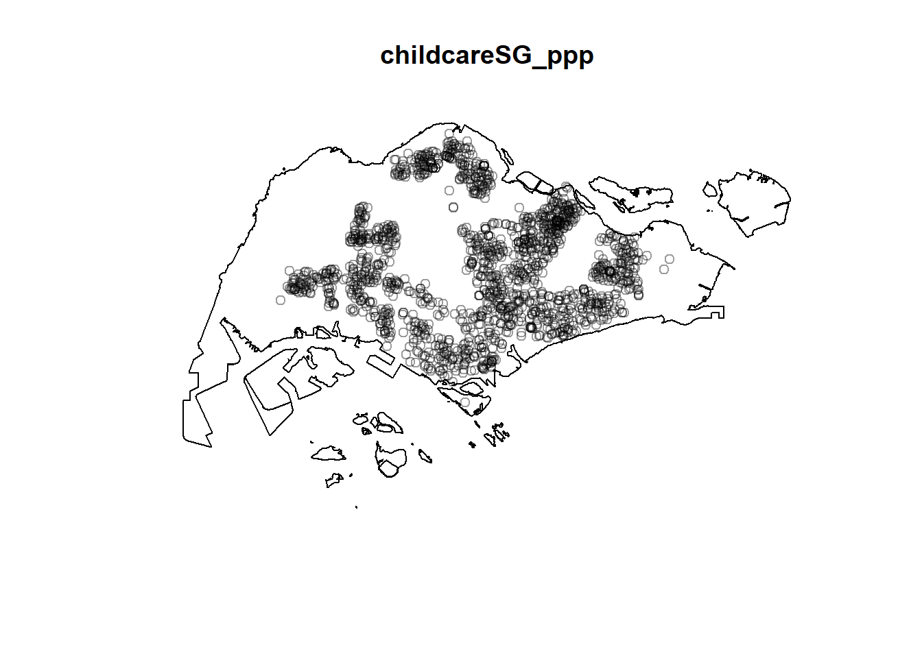

Mapping

tmap_mode("view")
tm_view(set.zoom.limits=c(10, 15)) +
tm_shape(childcare_sf) +  
  tm_dots(alpha=0.5)

KDE

Computing KDE using automatic bandwidth selection method

kde_childcareSG_bw <- density(childcareSG_ppp,
                              sigma=bw.diggle,
                              edge=TRUE,
                            kernel="gaussian")

plot(kde_childcareSG_bw)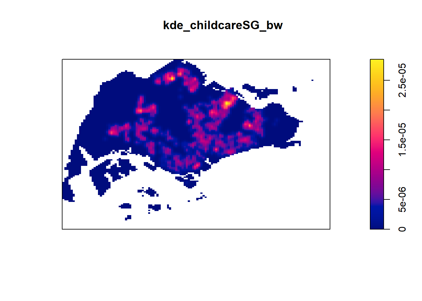

Bandwidth:

bw <- bw.diggle(childcareSG_ppp)
bw

   sigma 
298.4095

Rescaling KDE values

childcareSG_ppp.km <- rescale(childcareSG_ppp, 1000, "km")

kde_childcareSG.bw <- density(childcareSG_ppp.km, sigma=bw.diggle, edge=TRUE, kernel="gaussian")
plot(kde_childcareSG.bw)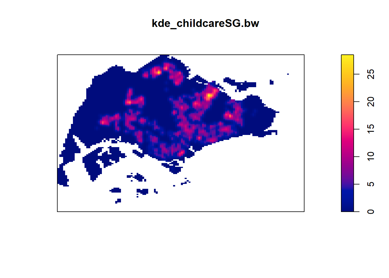

Different automatic bandwidth methods

bw.CvL(childcareSG_ppp.km)

   sigma 
4.543278

bw.scott(childcareSG_ppp.km)

 sigma.x  sigma.y 
2.224898 1.450966

bw.ppl(childcareSG_ppp.km)

    sigma 
0.3897114

bw.diggle(childcareSG_ppp.km)

    sigma 
0.2984095

bw.diggle vs bw.ppl

kde_childcareSG.ppl <- density(childcareSG_ppp.km, 
                               sigma=bw.ppl, 
                               edge=TRUE,
                               kernel="gaussian")
par(mfrow=c(1,2))
plot(kde_childcareSG.bw, main = "bw.diggle")
plot(kde_childcareSG.ppl, main = "bw.ppl")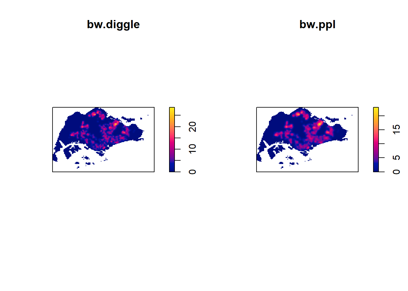

par(mfrow=c(2,2))
plot(density(childcareSG_ppp.km, 
             sigma=bw.ppl, 
             edge=TRUE, 
             kernel="gaussian"), 
     main="Gaussian")
plot(density(childcareSG_ppp.km, 
             sigma=bw.ppl, 
             edge=TRUE, 
             kernel="epanechnikov"), 
     main="Epanechnikov")
plot(density(childcareSG_ppp.km, 
             sigma=bw.ppl, 
             edge=TRUE, 
             kernel="quartic"), 
     main="Quartic")
plot(density(childcareSG_ppp.km, 
             sigma=bw.ppl, 
             edge=TRUE, 
             kernel="disc"), 
     main="Disc")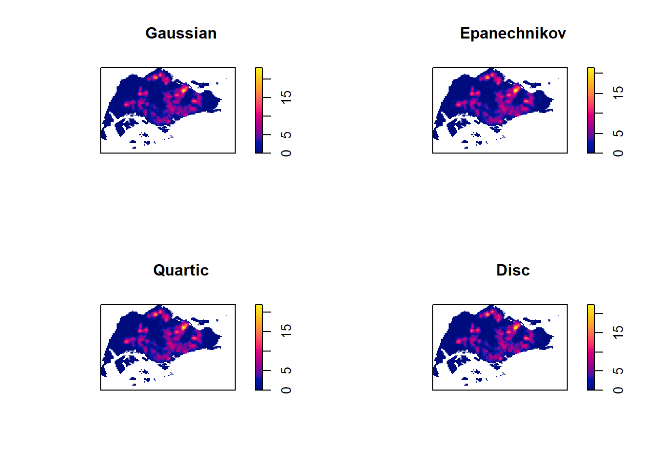

Fixed and Adaptive KDE

Fixed Bandwidth

kde_childcareSG_600 <- density(childcareSG_ppp.km, sigma=0.6, edge=TRUE, kernel="gaussian")
plot(kde_childcareSG_600)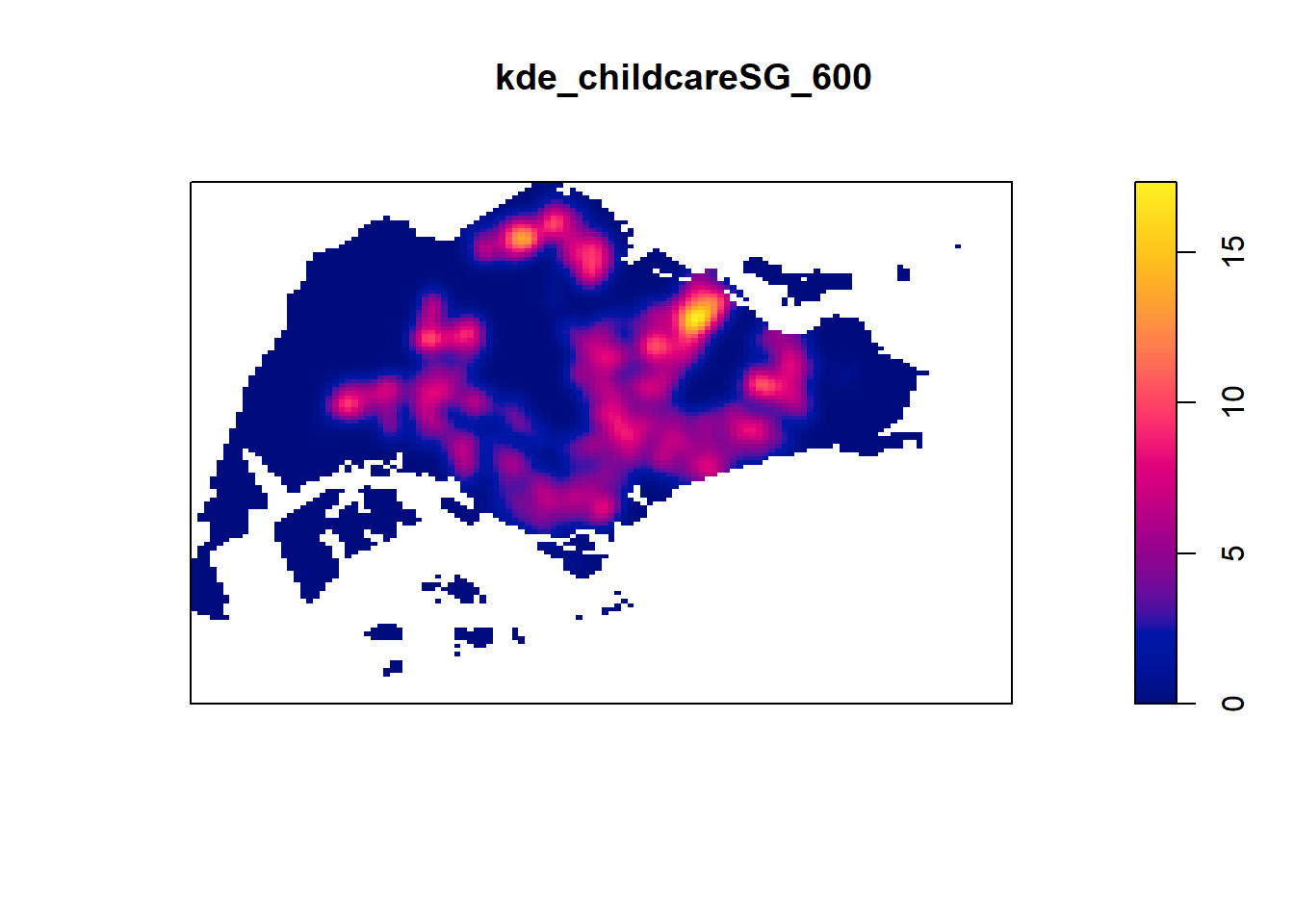

Adaptive Bandwidth

kde_childcareSG_adaptive <- adaptive.density(childcareSG_ppp.km, method="kernel")
plot(kde_childcareSG_adaptive)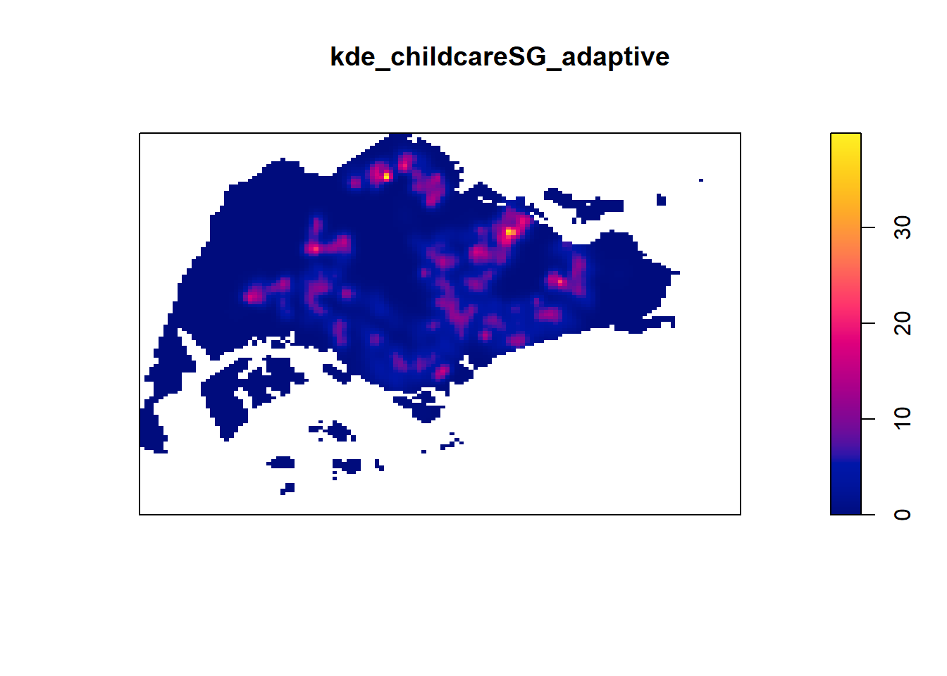

par(mfrow=c(1,2))
plot(kde_childcareSG.bw, main = "Fixed bandwidth")
plot(kde_childcareSG_adaptive, main = "Adaptive bandwidth")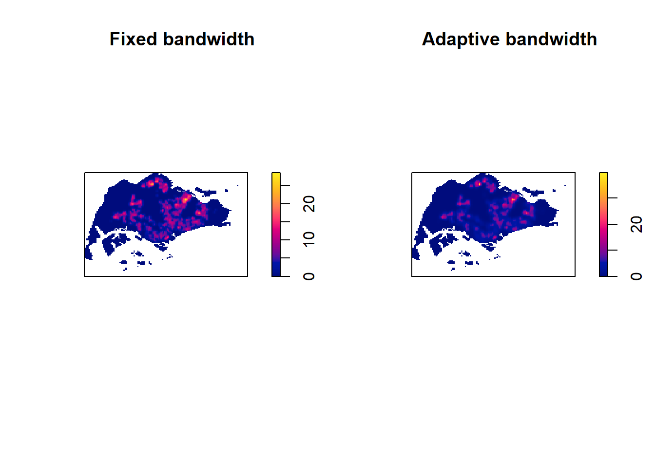

Converting KDE output into grid object

gridded_kde_childcareSG_bw <- as.SpatialGridDataFrame.im(kde_childcareSG.bw)
spplot(gridded_kde_childcareSG_bw)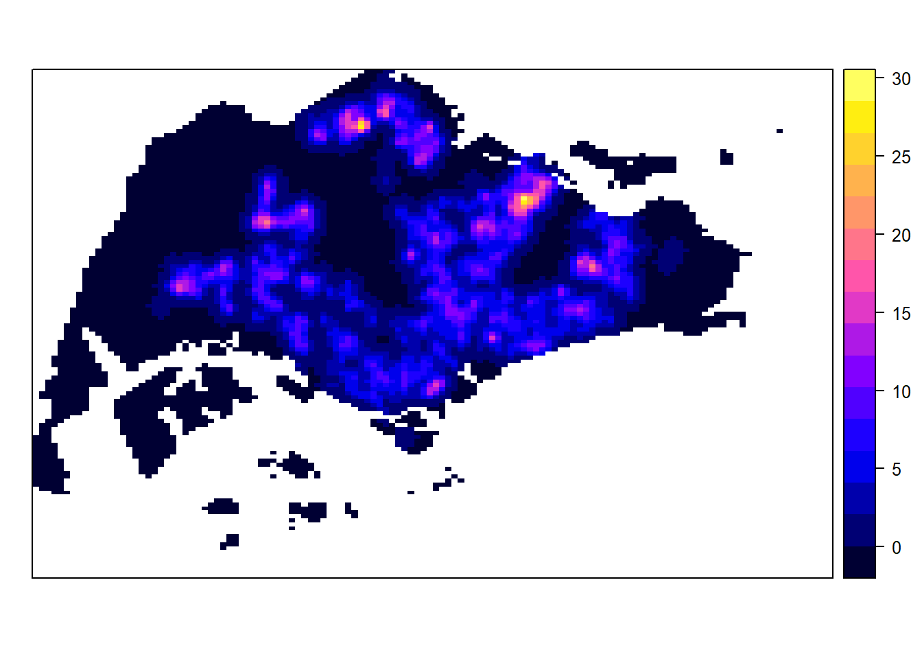

Converting into raster

kde_childcareSG_bw_raster <- raster(gridded_kde_childcareSG_bw)
kde_childcareSG_bw_raster

class      : RasterLayer 
dimensions : 128, 128, 16384  (nrow, ncol, ncell)
resolution : 0.4170614, 0.2647348  (x, y)
extent     : 2.663926, 56.04779, 16.35798, 50.24403  (xmin, xmax, ymin, ymax)
crs        : NA 
source     : memory
names      : v 
values     : -8.476185e-15, 28.51831  (min, max)

Assigning projection systems

projection(kde_childcareSG_bw_raster) <- CRS("+init=EPSG:3414 +units=km")
kde_childcareSG_bw_raster

class      : RasterLayer 
dimensions : 128, 128, 16384  (nrow, ncol, ncell)
resolution : 0.4170614, 0.2647348  (x, y)
extent     : 2.663926, 56.04779, 16.35798, 50.24403  (xmin, xmax, ymin, ymax)
crs        : +init=EPSG:3414 +units=km 
source     : memory
names      : v 
values     : -8.476185e-15, 28.51831  (min, max)

Plot in tmap

tm_shape(kde_childcareSG_bw_raster) + 
  tm_raster("v") +
  tm_layout(legend.position = c("right", "bottom"), frame = FALSE)