pacman::p_load(sf, tidyverse, tmap, maptools, raster, spatstat, sfdep)Take Home Exercise 1: Spatial Point Patterns Analysis on Nigerian Water Points
Background
Water is an important resource to mankind. However, despite its abundance on the planet, there are many who do not have access to clean water. In fact, according to UN-Water (2021), 2.3 billion people live in water-stressed countries.
This project aims to use data collected by Water Point Data Exchange (WPdx) to examine water points in Osun State, Nigeria, in hopes of being able to make inferences regarding their accessibility. As such, we are primarily concerned about the functional status of the water points, their distribution across the state, and possible correlations between functional and non-functional water points.
Import
Packages
The R packages used in this project are:
sf: for importing, managing, and processing geospatial data.
tidyverse: a family of other R packages for performing data science tasks such as importing, wrangling, and visualising data.
tmap: creating thematic maps
maptools: a set of tools for manipulating geographic data
raster: reads, writes, manipulates, analyses, and model gridded spatial data (raster)
spatstat: for performing spatial point patterns analysis
sfdep: for analysing spatial dependencies
Aspatial Data
The data we are going to use is from the WPdx Global Data Repositories, which is a collection of water point related data from rural areas. For this project, we are specifically looking at the WPdx+ data set, which is an enhanced version of the WPdx-Basic dataset.
As we are focused on the country of Nigeria, we will only be considering the data from Nigeria. We will also filter on the level-1 administrative boundary (state) of Osun.
wp_nga <- read_csv("data/aspatial/WPDX.csv") %>%
filter(`#clean_country_name` == "Nigeria", `#clean_adm1` == "Osun")Geospatial Data
This project will focus on the Osun State, Nigeria. We will get the state boundary GIS data of Nigeria from The Humanitarian Data Exchange portal.
osun <- st_read(dsn = "data/geospatial/NGA",
layer = "nga_admbnda_adm2_osgof_20190417") %>%
filter(`ADM1_EN` == "Osun") %>%
st_transform(crs = 26392)Reading layer `nga_admbnda_adm2_osgof_20190417' from data source
`C:\Jenpoer\IS415-GAA\Take-Home-Exercises\exe-01\data\geospatial\NGA'
using driver `ESRI Shapefile'
Simple feature collection with 774 features and 16 fields
Geometry type: MULTIPOLYGON
Dimension: XY
Bounding box: xmin: 2.668534 ymin: 4.273007 xmax: 14.67882 ymax: 13.89442
Geodetic CRS: WGS 84Data Preprocessing
Before we proceed with our analysis, we need to preprocess the data to the correct format and clean it.
Aspatial Data
Convert aspatial data to geospatial
To do some analysis on the data, we need to convert the aspatial data to geospatial data.
We need to convert wkt field into sfc field (i.e. simple feature object) by using st_as_sfc().
wp_nga$Geometry = st_as_sfc(wp_nga$`New Georeferenced Column`)
glimpse(wp_nga)Rows: 5,557
Columns: 71
$ row_id <dbl> 429123, 70566, 70578, 66401, 422190, 422…
$ `#source` <chr> "GRID3", "Federal Ministry of Water Reso…
$ `#lat_deg` <dbl> 8.020000, 7.317741, 7.759448, 8.031187, …
$ `#lon_deg` <dbl> 5.060000, 4.785507, 4.563998, 4.637400, …
$ `#report_date` <chr> "08/29/2018 12:00:00 AM", "05/11/2015 12…
$ `#status_id` <chr> "Unknown", "No", "No", "No", "Unknown", …
$ `#water_source_clean` <chr> NA, "Protected Shallow Well", "Borehole"…
$ `#water_source_category` <chr> NA, "Well", "Well", "Well", NA, NA, "Wel…
$ `#water_tech_clean` <chr> "Tapstand", "Mechanized Pump", "Mechaniz…
$ `#water_tech_category` <chr> "Tapstand", "Mechanized Pump", "Mechaniz…
$ `#facility_type` <chr> "Improved", "Improved", "Improved", "Imp…
$ `#clean_country_name` <chr> "Nigeria", "Nigeria", "Nigeria", "Nigeri…
$ `#clean_adm1` <chr> "Osun", "Osun", "Osun", "Osun", "Osun", …
$ `#clean_adm2` <chr> "Ifedayo", "Atakumosa East", "Osogbo", "…
$ `#clean_adm3` <chr> NA, NA, NA, NA, NA, NA, NA, NA, NA, NA, …
$ `#clean_adm4` <chr> NA, NA, NA, NA, NA, NA, NA, NA, NA, NA, …
$ `#install_year` <dbl> NA, NA, NA, 2004, NA, NA, 2006, 2014, 20…
$ `#installer` <chr> NA, NA, NA, NA, NA, NA, NA, NA, NA, NA, …
$ `#rehab_year` <lgl> NA, NA, NA, NA, NA, NA, NA, NA, NA, NA, …
$ `#rehabilitator` <lgl> NA, NA, NA, NA, NA, NA, NA, NA, NA, NA, …
$ `#management_clean` <chr> NA, NA, NA, NA, NA, NA, NA, NA, NA, "Com…
$ `#status_clean` <chr> NA, "Abandoned/Decommissioned", "Abandon…
$ `#pay` <chr> NA, "No", "No", "No", NA, NA, "No", "No"…
$ `#fecal_coliform_presence` <chr> NA, NA, NA, NA, NA, NA, NA, NA, NA, NA, …
$ `#fecal_coliform_value` <dbl> NA, NA, NA, NA, NA, NA, NA, NA, NA, NA, …
$ `#subjective_quality` <chr> NA, "Acceptable quality", "Acceptable qu…
$ `#activity_id` <chr> "6054e946-2573-45bf-ab7c-0ddaa68a61b4", …
$ `#scheme_id` <chr> NA, NA, NA, NA, NA, NA, NA, NA, NA, NA, …
$ `#wpdx_id` <chr> "6FW723C6+222", "6FV68Q9P+36R", "6FV6QH5…
$ `#notes` <chr> "Rt Hon Kola Oluwawole Water Tap", "Temi…
$ `#orig_lnk` <chr> "https://nigeria.africageoportal.com/dat…
$ `#photo_lnk` <chr> NA, "https://akvoflow-55.s3.amazonaws.co…
$ `#country_id` <chr> "NG", "NG", "NG", "NG", "NG", "NG", "NG"…
$ `#data_lnk` <chr> "https://catalog.waterpointdata.org/data…
$ `#distance_to_primary_road` <dbl> 4474.22234, 10130.42742, 167.82235, 4133…
$ `#distance_to_secondary_road` <dbl> 1883.98780, 17466.35720, 838.91849, 1162…
$ `#distance_to_tertiary_road` <dbl> 1885.874322, 2376.832183, 1181.107236, 9…
$ `#distance_to_city` <dbl> 40100.268, 31549.222, 2449.293, 16704.19…
$ `#distance_to_town` <dbl> 8120.871, 24652.907, 9463.295, 5176.899,…
$ water_point_history <chr> "{\"2018-08-29\": {\"source\": \"GRID3\"…
$ rehab_priority <dbl> NA, NA, NA, NA, NA, NA, NA, NA, NA, NA, …
$ water_point_population <dbl> NA, NA, NA, NA, NA, NA, NA, NA, 0, 508, …
$ local_population_1km <dbl> NA, NA, NA, NA, NA, NA, NA, NA, 70, 647,…
$ crucialness_score <dbl> NA, NA, NA, NA, NA, NA, NA, NA, NA, 0.78…
$ pressure_score <dbl> NA, NA, NA, NA, NA, NA, NA, NA, NA, 1.69…
$ usage_capacity <dbl> 250, 1000, 1000, 1000, 250, 250, 1000, 3…
$ is_urban <lgl> FALSE, FALSE, TRUE, FALSE, FALSE, FALSE,…
$ days_since_report <dbl> 1483, 2689, 2689, 2700, 1483, 1483, 2688…
$ staleness_score <dbl> 62.65911, 42.84384, 42.84384, 42.69554, …
$ latest_record <lgl> TRUE, TRUE, TRUE, TRUE, TRUE, TRUE, TRUE…
$ location_id <dbl> 358783, 239555, 239556, 230405, 358062, …
$ cluster_size <dbl> 1, 1, 1, 1, 1, 1, 1, 1, 1, 1, 1, 1, 1, 1…
$ `#clean_country_id` <chr> "NGA", "NGA", "NGA", "NGA", "NGA", "NGA"…
$ `#country_name` <chr> "Nigeria", "Nigeria", "Nigeria", "Nigeri…
$ `#water_source` <chr> "Tap", "Improved Protected dug well", "I…
$ `#water_tech` <chr> NA, "Motorised", "Motorised", "Motorised…
$ `#status` <chr> NA, "Non-functional Abandoned", "Non-fun…
$ `#adm2` <chr> NA, "Atakumosa East", "Osogbo", "Odo-Oti…
$ `#adm3` <chr> NA, NA, NA, NA, NA, NA, NA, NA, NA, NA, …
$ `#management` <chr> NA, NA, NA, NA, NA, NA, NA, NA, NA, "Com…
$ `#adm1` <chr> NA, "Osun", "Osun", "Osun", NA, NA, "Osu…
$ `New Georeferenced Column` <chr> "POINT (5.06 8.02)", "POINT (4.7855068 7…
$ lat_deg_original <dbl> NA, NA, NA, NA, NA, NA, NA, NA, NA, NA, …
$ lat_lon_deg <chr> "(8.02°, 5.06°)", "(7.3177411°, 4.785506…
$ lon_deg_original <dbl> NA, NA, NA, NA, NA, NA, NA, NA, NA, NA, …
$ public_data_source <chr> "https://catalog.waterpointdata.org/data…
$ converted <chr> NA, "#status_id, #water_source, #pay, #s…
$ count <dbl> 1, 1, 1, 1, 1, 1, 1, 1, 1, 1, 1, 1, 1, 1…
$ created_timestamp <chr> "12/06/2021 09:12:57 PM", "06/30/2020 12…
$ updated_timestamp <chr> "12/06/2021 09:12:57 PM", "06/30/2020 12…
$ Geometry <POINT> POINT (5.06 8.02), POINT (4.785507 7.3…We need to use EPSG 4326 because we want to put back the projection information first, as it is from aspatial data.
wp_sf <- st_sf(wp_nga, crs=4326)
st_geometry(wp_sf)Geometry set for 5557 features
Geometry type: POINT
Dimension: XY
Bounding box: xmin: 4.032004 ymin: 7.060309 xmax: 5.06 ymax: 8.061898
Geodetic CRS: WGS 84
First 5 geometries:Inspecting the newly created dataframe, we find that it’s using the WGS84 coordinate system. We need to project it to Nigeria’s projected coordinate system.
wp_sf <- wp_sf %>%
st_transform(crs = 26392)Selecting and cleaning relevant information
According to the documentation in the WPdx repository, the #status_clean column denotes a categorized version of the #status column, which tells us the physical / mechanical condition of the water point (i.e. whether or not it is functional). As such, we will primarily be working with this column. We can rename the column so that it’s more readable.
wp_sf <- wp_sf %>%
rename(status_clean = '#status_clean')Now, let’s visualise the possible categories that this column contains!
unique(wp_sf$`status_clean`)[1] NA "Abandoned/Decommissioned"
[3] "Functional but needs repair" "Functional"
[5] "Functional but not in use" "Abandoned"
[7] "Non-Functional" "Non-Functional due to dry season"There are NA values present in the column. Ideally, we want to replace these values with a category so that they do not interfere with calculations.
wp_sf <- wp_sf %>%
mutate(status_clean = replace_na(
status_clean, "Unknown"
))Visualising the possible categories once more, we can see that all the NA values have been replaced to Unknown.
unique(wp_sf$`status_clean`)[1] "Unknown" "Abandoned/Decommissioned"
[3] "Functional but needs repair" "Functional"
[5] "Functional but not in use" "Abandoned"
[7] "Non-Functional" "Non-Functional due to dry season"To make it easier to work with the data, let’s only select columns that we need, namely:
clean_country_name: country name the data is derived from (Nigeria), simply retained for reference
clean_adm1: name of the state we are concerned with (Osun), simply retained for reference
clean_adm2: names of level-2 administrative boundary (LGA)
Geometry: the geospatial information that we generated from the aspatial data
status_clean: the statuses of the water points
In addition, we want to constrain the water points to only those that are within the Osun region defined by the state boundary GIS data.
wp_sf_osun <- wp_sf %>%
st_intersection(osun) %>%
dplyr::select(c("Geometry", "status_clean", "X.clean_country_name", "X.clean_adm1", "X.clean_adm2")) %>%
rename(clean_country_name = 'X.clean_country_name',
clean_adm1 = 'X.clean_adm1',
clean_adm2 = 'X.clean_adm2')
glimpse(wp_sf_osun)Rows: 5,322
Columns: 5
$ Geometry <POINT [m]> POINT (212810 386707.6), POINT (212202 349210…
$ status_clean <chr> "Functional but needs repair", "Functional", "Funct…
$ clean_country_name <chr> "Nigeria", "Nigeria", "Nigeria", "Nigeria", "Nigeri…
$ clean_adm1 <chr> "Osun", "Osun", "Osun", "Osun", "Osun", "Osun", "Os…
$ clean_adm2 <chr> "Aiyedade", "Aiyedade", "Aiyedade", "Aiyedade", "Ai…Geospatial Data
Selecting relevant information
To make our data easier to work with, we will select only the relevant columns of the geospatial data, which are:
ADM2_EN: English name of the level-2 administrative boundary (LGA)
ADM2_PCODE: code for the level-2 administrative boundary (LGA)
ADM1_EN: English name of the level-1 administrative boundary (state); in this case, Osun. The information is retained for reference.
ADM1_PCODE: code for the level-1 administrative boundary (state); in this case, NG030. The information is retained for reference.
geometry: the geospatial information
osun <- osun %>% dplyr::select(c(3:4, 8:9))Deriving additional columns
We are also concerned with the proportions of functional and non-functional water points to view their distributions. Hence, we will derive additional columns for this information and attach them to the geospatial data.
Add a column called func_status
The func_status column will categorize the status_clean column into “Functional”, “Non-Functional”, and “Unknown” instead of the 7 different categories.
wp_sf_osun <- wp_sf_osun %>%
mutate(`func_status` = case_when(
`status_clean` %in% c("Functional",
"Functional but not in use",
"Functional but needs repair") ~
"Functional",
`status_clean` %in% c("Abandoned/Decommissioned",
"Non-Functional due to dry season",
"Non-Functional",
"Abandoned",
"Non functional due to dry season") ~
"Non-Functional",
`status_clean` == "Unknown" ~ "Unknown"))Frequency of functional water points
functional <- wp_sf_osun %>%
filter(`func_status` == "Functional")
osun$`wp_functional` <- lengths(st_intersects(osun, functional))Frequency of non-functional water points
non_functional <- wp_sf_osun %>%
filter(`func_status` == "Non-Functional")
osun$`wp_non_functional` <- lengths(st_intersects(osun, non_functional))Frequency of unknown status water points
unknown <- wp_sf_osun %>%
filter(`func_status` == "Unknown")
osun$`wp_unknown` <- lengths(st_intersects(osun, unknown))Total frequency of water points
osun$`wp_total` <- lengths(st_intersects(osun, wp_sf_osun))Calculate proportions of functional and non-functional water points
The proportions of functional and non-functional water points are calculated by dividing their respective frequencies with the total frequency of water points.
osun <- osun %>%
mutate(`prop_functional` = `wp_functional`/`wp_total`,
`prop_non_functional` = `wp_non_functional`/`wp_total`)Converting sf data frame to spatstat objects
In order to do spatial patterns points analysis, we will be using the spatstat package. However, we must first convert our data, which is currently in the form of sf data frames into the appropriate data types. As of this point, there are no direct conversions. Hence, we must do several intermediate steps.
1) Convert sf data frames to sp’s Spatial* class
osun_spatial <- as_Spatial(osun)
wp_spatial <- as_Spatial(wp_sf_osun)
func_spatial <- as_Spatial(functional)
non_func_spatial <- as_Spatial(non_functional)2) Converting Spatial* class into generic sp format
osun_sp <- as(osun_spatial, "SpatialPolygons")
wp_sp <- as(wp_spatial, "SpatialPoints")
func_sp <- as(func_spatial, "SpatialPoints")
non_func_sp <- as(non_func_spatial, "SpatialPoints")3) Converting generic sp format into spatstat’s ppp format
wp_ppp <- as(wp_sp, "ppp")
func_ppp <- as(func_sp, "ppp")
non_func_ppp <- as(non_func_sp, "ppp")Let’s visualise all the water point data in the ppp format.
plot(wp_ppp)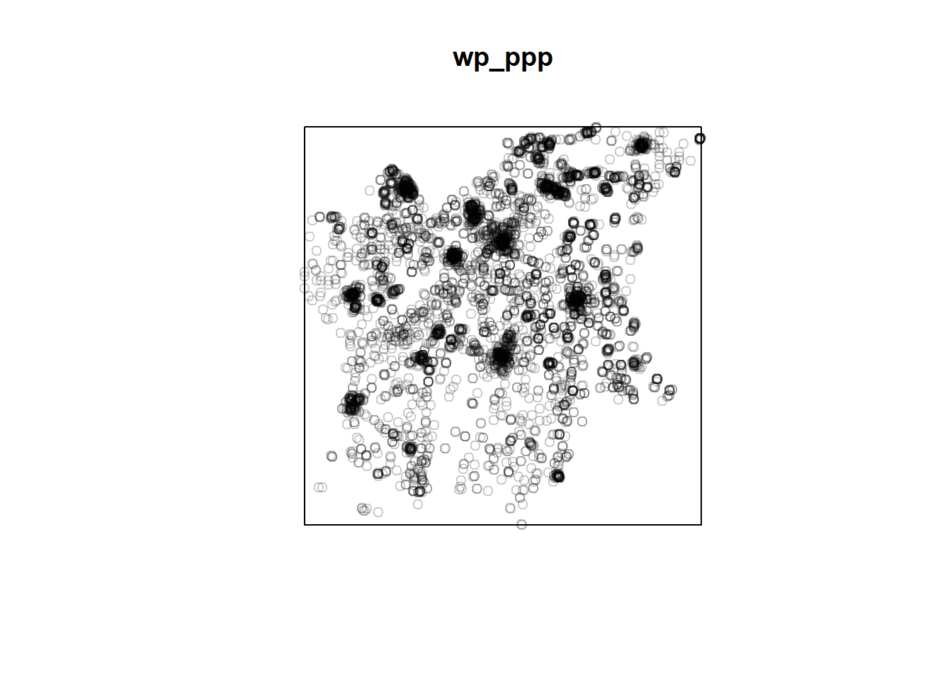
We can take a look at the summary statistics of the newly created ppp objects.
summary(wp_ppp)Planar point pattern: 5322 points
Average intensity 4.352014e-07 points per square unit
Coordinates are given to 2 decimal places
i.e. rounded to the nearest multiple of 0.01 units
Window: rectangle = [180388.11, 290750.96] x [340054.1, 450859.7] units
(110400 x 110800 units)
Window area = 12228800000 square unitssummary(func_ppp)Planar point pattern: 2529 points
Average intensity 2.197764e-07 points per square unit
Coordinates are given to 2 decimal places
i.e. rounded to the nearest multiple of 0.01 units
Window: rectangle = [183479.97, 290750.96] x [343587.9, 450859.7] units
(107300 x 107300 units)
Window area = 11507100000 square unitssummary(non_func_ppp)Planar point pattern: 2059 points
Average intensity 1.719992e-07 points per square unit
Coordinates are given to 2 decimal places
i.e. rounded to the nearest multiple of 0.01 units
Window: rectangle = [182502.44, 290616] x [340054.1, 450780.1] units
(108100 x 110700 units)
Window area = 1.1971e+10 square units4) Creating owin object
We need to confine our analysis to the Osun State boundary using spatstat’s owin object, which is specially designed to represent polygonal regions.
osun_owin <- as(osun_sp, "owin")plot(osun_owin)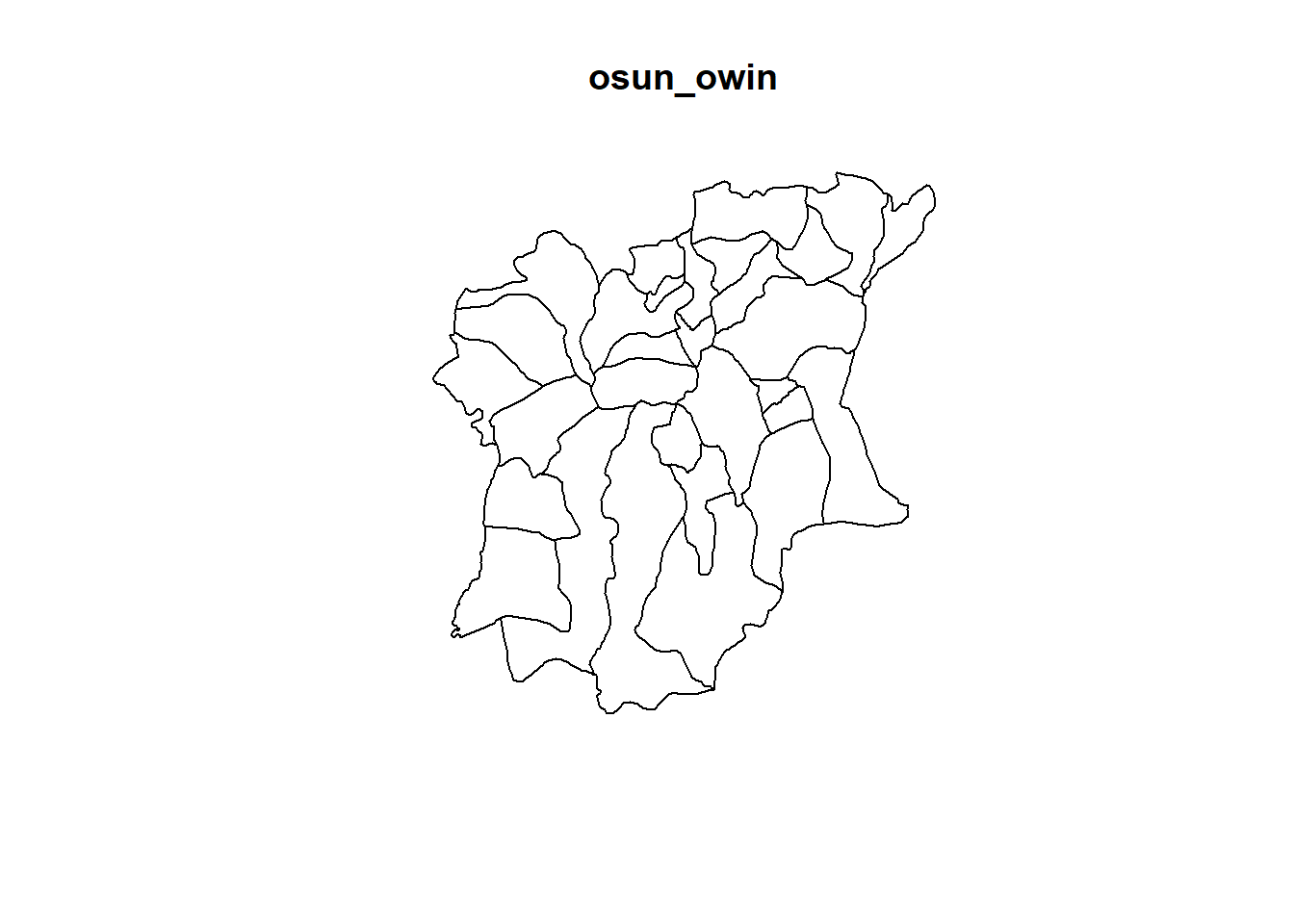
summary(osun_owin)Window: polygonal boundary
30 separate polygons (no holes)
vertices area relative.area
polygon 1 204 766084000 0.08870
polygon 2 81 304399000 0.03520
polygon 3 97 465688000 0.05390
polygon 4 124 373051000 0.04320
polygon 5 60 149473000 0.01730
polygon 6 84 144820000 0.01680
polygon 7 50 102243000 0.01180
polygon 8 72 216002000 0.02500
polygon 9 112 269897000 0.03130
polygon 10 125 365142000 0.04230
polygon 11 83 111191000 0.01290
polygon 12 126 192557000 0.02230
polygon 13 219 904397000 0.10500
polygon 14 174 741131000 0.08580
polygon 15 81 138742000 0.01610
polygon 16 65 119452000 0.01380
polygon 17 90 280205000 0.03240
polygon 18 69 69814600 0.00808
polygon 19 69 42727500 0.00495
polygon 20 49 30458800 0.00353
polygon 21 62 263505000 0.03050
polygon 22 93 438930000 0.05080
polygon 23 87 274127000 0.03170
polygon 24 105 509979000 0.05910
polygon 25 98 292058000 0.03380
polygon 26 64 327765000 0.03800
polygon 27 133 108945000 0.01260
polygon 28 122 462169000 0.05350
polygon 29 94 109715000 0.01270
polygon 30 95 61239800 0.00709
enclosing rectangle: [176503.22, 291043.82] x [331434.7, 454520.1] units
(114500 x 123100 units)
Window area = 8635910000 square units
Fraction of frame area: 0.613Combining point events object and owin object
We can combine the ppp object of the water points with the owin object of Osun’s boundary.
wp_osun_ppp = wp_ppp[osun_owin]
wp_osun_func_ppp = func_ppp[osun_owin]
wp_osun_non_func_ppp = non_func_ppp[osun_owin]summary(wp_osun_ppp)Planar point pattern: 5322 points
Average intensity 6.162642e-07 points per square unit
Coordinates are given to 2 decimal places
i.e. rounded to the nearest multiple of 0.01 units
Window: polygonal boundary
30 separate polygons (no holes)
vertices area relative.area
polygon 1 204 766084000 0.08870
polygon 2 81 304399000 0.03520
polygon 3 97 465688000 0.05390
polygon 4 124 373051000 0.04320
polygon 5 60 149473000 0.01730
polygon 6 84 144820000 0.01680
polygon 7 50 102243000 0.01180
polygon 8 72 216002000 0.02500
polygon 9 112 269897000 0.03130
polygon 10 125 365142000 0.04230
polygon 11 83 111191000 0.01290
polygon 12 126 192557000 0.02230
polygon 13 219 904397000 0.10500
polygon 14 174 741131000 0.08580
polygon 15 81 138742000 0.01610
polygon 16 65 119452000 0.01380
polygon 17 90 280205000 0.03240
polygon 18 69 69814600 0.00808
polygon 19 69 42727500 0.00495
polygon 20 49 30458800 0.00353
polygon 21 62 263505000 0.03050
polygon 22 93 438930000 0.05080
polygon 23 87 274127000 0.03170
polygon 24 105 509979000 0.05910
polygon 25 98 292058000 0.03380
polygon 26 64 327765000 0.03800
polygon 27 133 108945000 0.01260
polygon 28 122 462169000 0.05350
polygon 29 94 109715000 0.01270
polygon 30 95 61239800 0.00709
enclosing rectangle: [176503.22, 291043.82] x [331434.7, 454520.1] units
(114500 x 123100 units)
Window area = 8635910000 square units
Fraction of frame area: 0.613plot(wp_osun_ppp)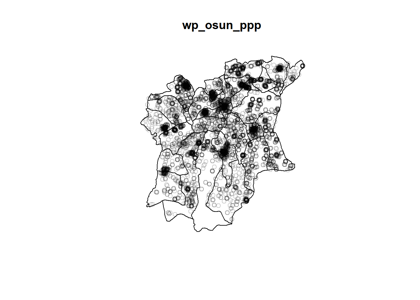
Exploratory Data Analysis
Before we begin with statistical analysis, let us first do some exploratory data analysis by visualising the distribution of the spatial point events (namely, the water points in Osun).
Point Map
First, let’s visualise the distribution of all water points in the state of Osun. As water points are considered spatial point events, we can use a point map to illustrate their occurrence.
tmap_mode("view")
tm_basemap("OpenStreetMap") +
tm_view(set.zoom.limits=c(8, 18)) +
tm_shape(osun) +
tm_borders(lwd=0.5) +
tm_shape(wp_sf_osun) +
tm_dots(title = "Status", col = "func_status", alpha = 0.7) +
tm_layout(main.title="Distribution of All Water Points")We can see several areas where many points seem to be gathered together. Since we are concerned about the distribution of functional and non-functional water points, let us also visualise their distributions separately side-by-side using a facet map.
tmap_mode("plot")func_points <- tm_shape(osun) +
tm_fill() +
tm_shape(functional) +
tm_dots() +
tm_layout(main.title="Distribution of Functional Water Points",
main.title.size = 1)non_func_points <- tm_shape(osun) +
tm_fill() +
tm_shape(non_functional) +
tm_dots() +
tm_layout(main.title="Distribution of Non-Functional Water Points",
main.title.size = 1)tmap_arrange(func_points, non_func_points, nrow = 1)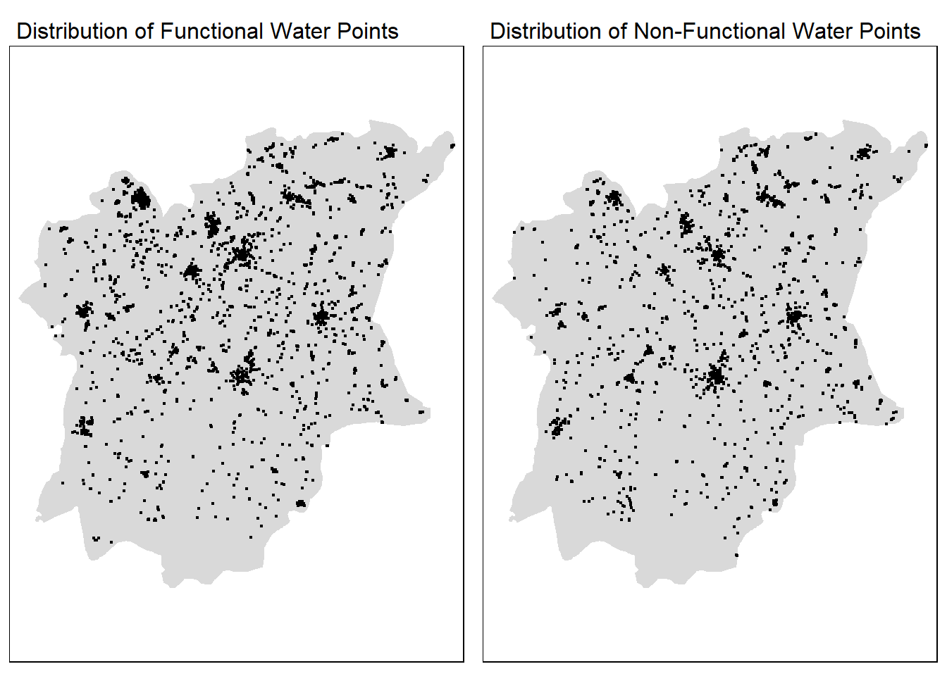
Although we can also pinpoint areas where many points seem to be gathered together, it’s rather hard to pinpoint their density relative to each other.
Choropleth Map of Rate per LGA
Since we have calculated proportions of the functional and non-functional water points per LGA, we can use a choropleth map to visualise their distribution by LGA as well.
func_rate_lga <- tm_shape(osun) +
tm_fill("prop_functional",
n = 10,
title="Proportion",
style = "equal",
palette = "Blues") +
tm_borders(lwd = 0.1,
alpha = 1) +
tm_layout(main.title = "Distribution of functional water points",
legend.outside = FALSE,
main.title.size = 1)non_func_rate_lga <- tm_shape(osun) +
tm_fill("prop_non_functional",
n = 10,
title="Proportion",
style = "equal",
palette = "Blues") +
tm_borders(lwd = 0.1,
alpha = 1) +
tm_layout(main.title = "Distribution of non-functional water points",
legend.outside = FALSE,
main.title.size = 1)tmap_arrange(func_rate_lga, non_func_rate_lga, nrow=1)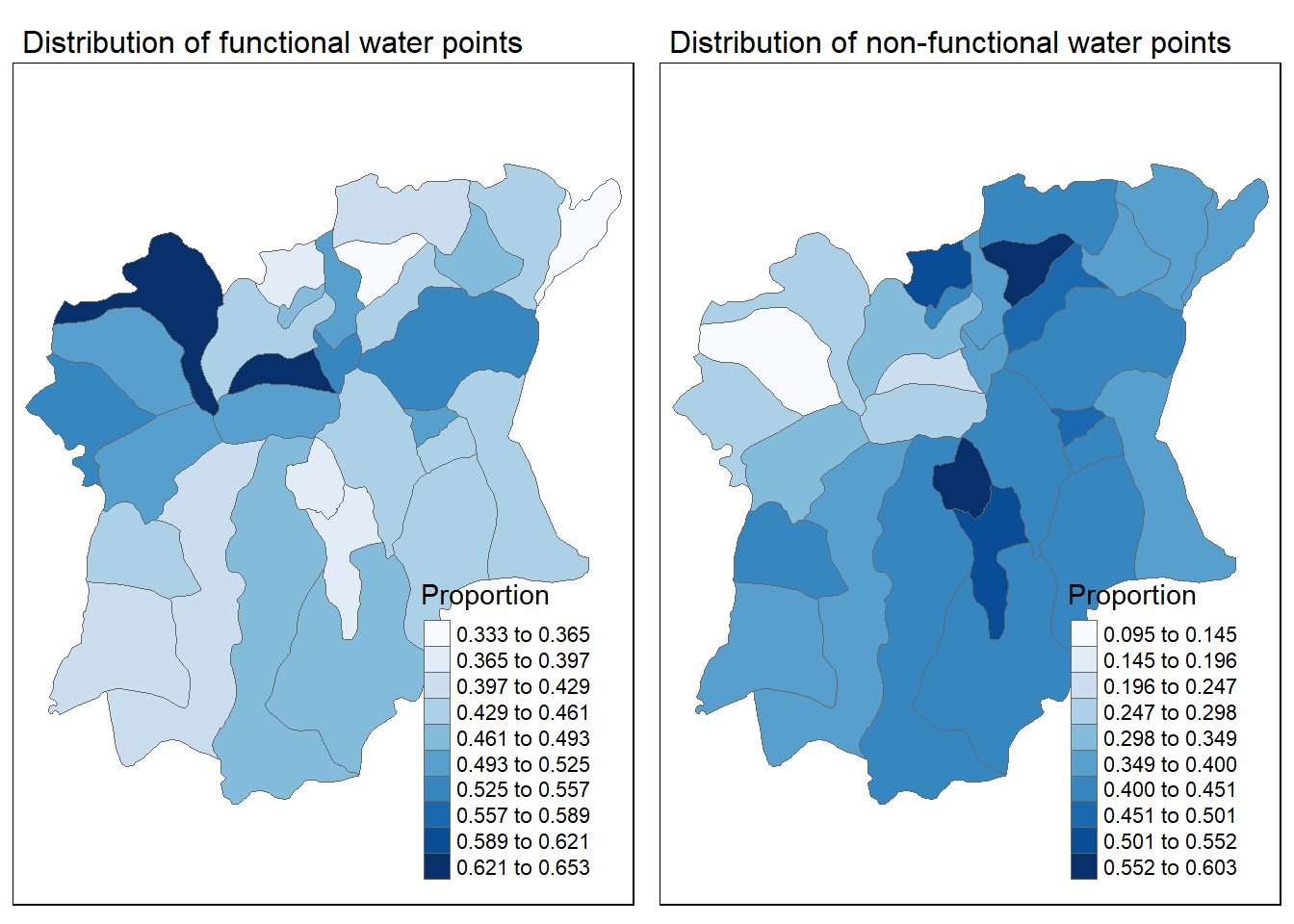
This allows us to see which LGAs have the highest proportion of functional water points and which LGAs have the highest proportion of non-functional water points. However, with these choropleth maps, we are constrained to viewing the data by LGAs.
Kernel Density Estimation
If we want to better visualise areas of high density without being constrained to viewing them in terms of LGAs, we can use kernel density estimation.
Automatic bandwidth selection
First of all, we will rescale the data to kilometers.
wp_osun_ppp.km <- rescale(wp_osun_ppp, 1000, "km")
wp_osun_func_ppp.km <- rescale(wp_osun_func_ppp, 1000, "km")
wp_osun_non_func_ppp.km <- rescale(wp_osun_non_func_ppp, 1000, "km")Then, we can automatically calculate bandwidth using spatstat’s bw.diggle and bw.ppl functions, which will perform the cross-validation to select an appropriate bandwidth for the kernel density estimation.
kde_wp_osun_bw.diggle <- density(wp_osun_ppp.km,
sigma=bw.diggle,
edge=TRUE,
kernel="gaussian")
kde_wp_osun_bw.ppl <- density(wp_osun_ppp.km,
sigma=bw.ppl,
edge=TRUE,
kernel="gaussian")The bandwidth selected by the bw.diggle function is:
bw.diggle(wp_osun_ppp.km) sigma
0.2223774 The bandwidth selected by the bw.ppl function is:
bw.ppl(wp_osun_ppp.km) sigma
0.4905715 par(mfrow=c(1,2))
plot(kde_wp_osun_bw.diggle, main="diggle")
plot(kde_wp_osun_bw.ppl, main="ppl")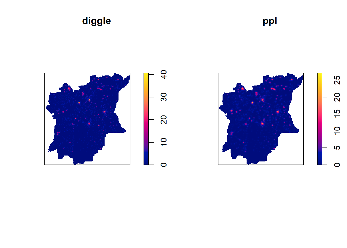
The bw.ppl function tends to select a larger bandwidth than the bw.diggle function. According to Baddeley et. (2016), the bw.ppl algorithm tends to produce more appropriate values when the pattern consists of predominantly tight clusters. However, bw.diggle works better to detect a single tight cluster in the midst of random noise.
Since the purpose of this project is to visualise where all the clusters of water points are in the state of Osun, the bw.ppl algorithm seems to be more appropriate. As can be seen from the plots as well, it seems to give us a clearer picture on the areas of high point density. Hence, from this point on, we will be using bw.ppl.
kde_wp_osun_func_bw <- density(wp_osun_func_ppp.km,
sigma=bw.ppl,
edge=TRUE,
kernel="gaussian")
kde_wp_osun_non_func_bw <- density(wp_osun_non_func_ppp.km,
sigma=bw.ppl,
edge=TRUE,
kernel="gaussian")Selected bandwidth for functional water points:
bw.ppl(wp_osun_func_ppp.km) sigma
0.9192953 Selected bandwidth for non-functional water points:
bw.ppl(wp_osun_non_func_ppp.km) sigma
0.9737385 par(mfrow=c(1,2))
plot(kde_wp_osun_func_bw, main="Functional")
plot(kde_wp_osun_non_func_bw, main="Non-Functional")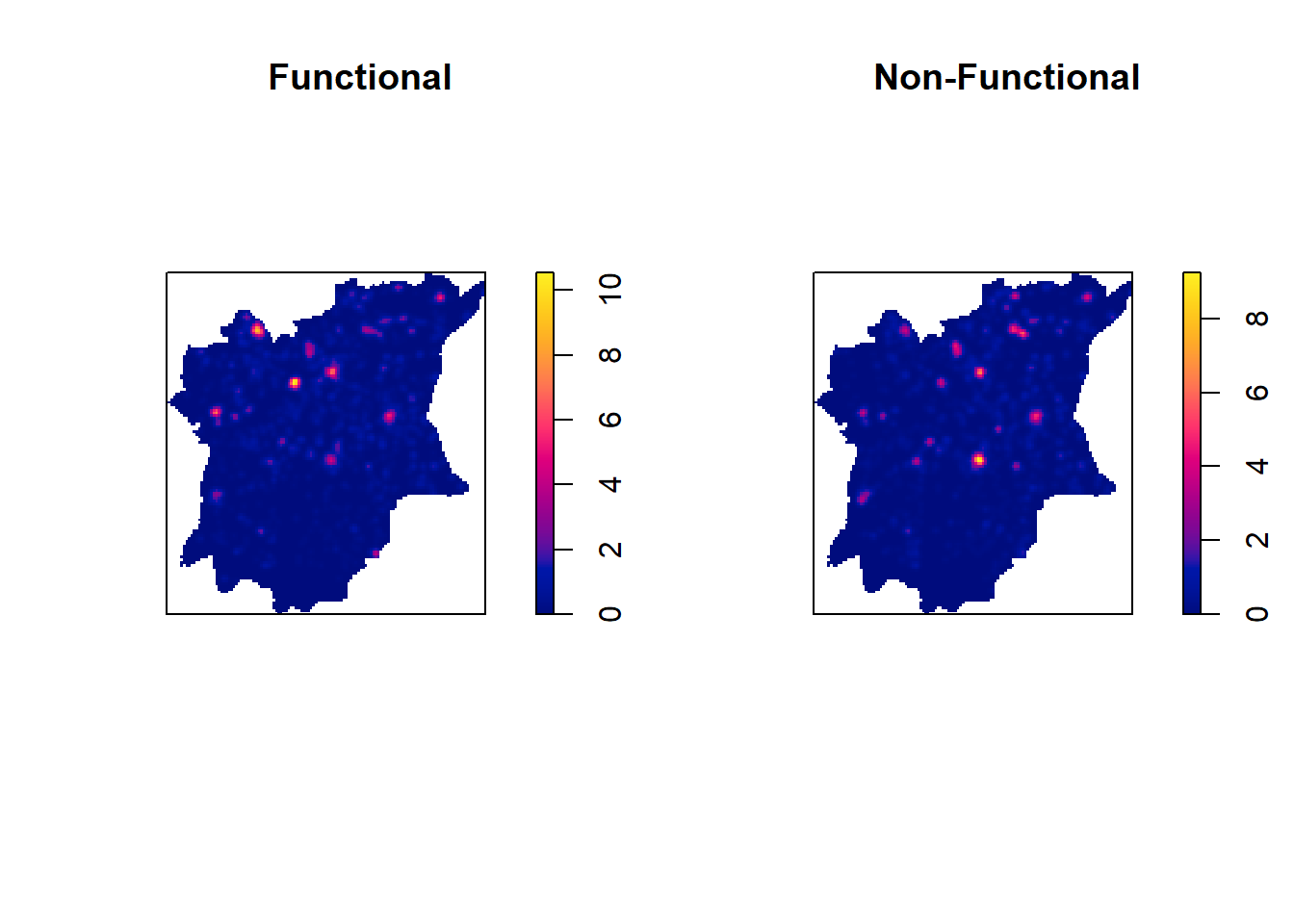
Mapping
To use the tmap package to plot the results of our kernel density estimation, we need to convert the data to the appropriate format.
1) Convert the KDE output into grid object
grid_kde_wp_osun_bw <- as.SpatialGridDataFrame.im(kde_wp_osun_bw.ppl)
grid_kde_wp_osun_func_bw <- as.SpatialGridDataFrame.im(kde_wp_osun_func_bw)
grid_kde_wp_osun_non_func_bw <- as.SpatialGridDataFrame.im(kde_wp_osun_non_func_bw)2) Convert grid objects into raster
raster_kde_wp_osun_bw <- raster(grid_kde_wp_osun_bw)
raster_kde_wp_osun_func_bw <- raster(grid_kde_wp_osun_func_bw)
raster_kde_wp_osun_non_func_bw <- raster(grid_kde_wp_osun_non_func_bw)We have to re-assign the correct projection systems onto the raster objects. We use EPSG 26392 for the Nigerian projection system and units km because we rescaled the data when computing the KDE.
crs(raster_kde_wp_osun_bw) <- CRS("+init=EPSG:26392 +units=km")
crs(raster_kde_wp_osun_func_bw) <- CRS("+init=EPSG:26392 +units=km")
crs(raster_kde_wp_osun_non_func_bw) <- CRS("+init=EPSG:26392 +units=km")Now, we can finally start mapping our raster objects!
Let’s visualise the KDE plot of all the water points on an interactive openstreetmap.
tmap_mode("view")
tm_basemap("OpenStreetMap") +
tm_view(set.zoom.limits=c(8, 18)) +
tm_shape(raster_kde_wp_osun_bw) +
tm_raster("v", palette = "YlGnBu", title="", alpha=0.7)Now, we can visualise the kernel density maps of functional and non-functional water points side by side.
tmap_mode("plot")map_kde_func <- tm_shape(raster_kde_wp_osun_func_bw) +
tm_raster("v", palette = "YlGnBu", title="") +
tm_layout(
legend.position = c("right", "bottom"),
main.title = "Functional",
frame = FALSE
)map_kde_non_func <- tm_shape(raster_kde_wp_osun_non_func_bw) +
tm_raster("v", palette = "YlOrRd", title="") +
tm_layout(
legend.position = c("right", "bottom"),
main.title = "Non-Functional",
frame = FALSE
)tmap_arrange(map_kde_func, map_kde_non_func, nrow = 1)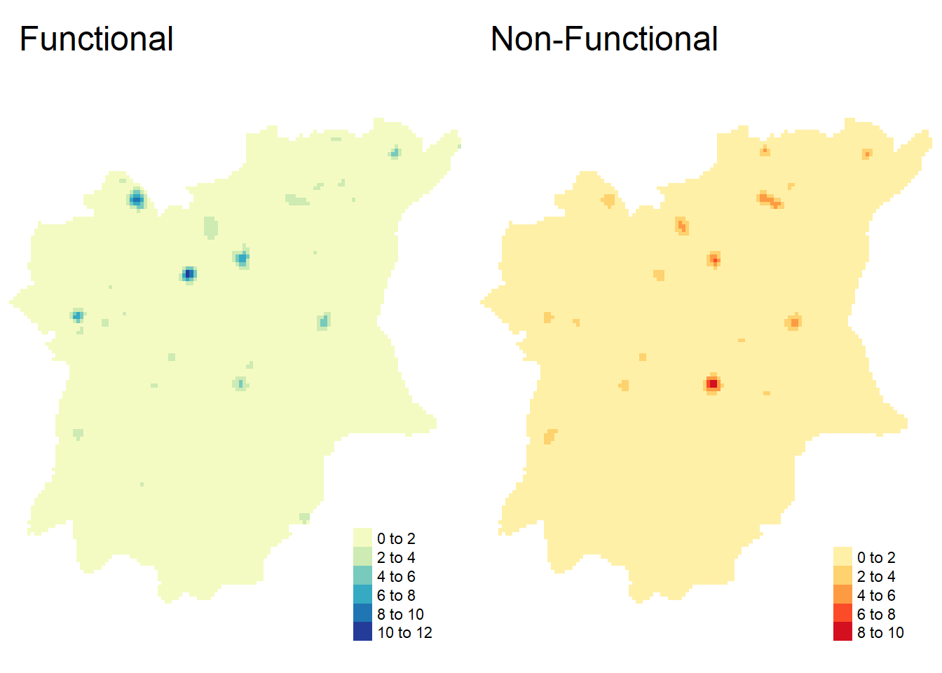
Analysis
From the plots, we can see that the functional water points seem to be clustered around northern Osun (in LGAs such as Ejigbo, Ede North, Osogbo), whereas the non-functional water points seem to be clustered around southern / central Osun (in LGAs such as Ife Central, Ife East, Ilesha West, Ilesha East).
As a whole, the water points themselves seem to be unevenly distributed, with northern Osun having more water points as a whole and southern Osun being more sparse.
Reference for LGAs:
lga_kde_func <- map_kde_func +
tm_shape(osun) +
tm_borders() +
tm_text("ADM2_EN", size = 0.6)
lga_kde_non_func <- map_kde_non_func +
tm_shape(osun) +
tm_borders() +
tm_text("ADM2_EN", size = 0.6)
tmap_arrange(lga_kde_func, lga_kde_non_func, nrow = 1)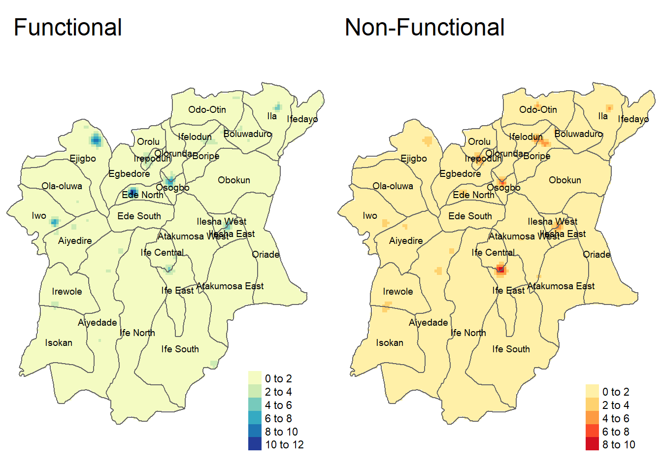
Comparison to point map
tmap_arrange(map_kde_func, map_kde_non_func, func_points, non_func_points,
nrow = 2, ncol = 2)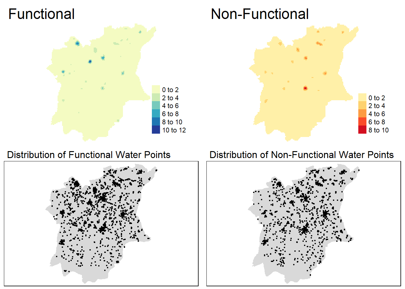
Compared to the point map, we can see that the KDE maps have the advantage of clearly pinpointing areas of high point density. We do not have to manually discern with our own eyes which areas seem to have a lot of points gathered together, because the KDE maps color-codes them in a gradient. Therefore, we can make comparisons between the distribution of the points more easily by looking at the intensity of the colors, instead of making guesses based on the number of points we can see.
However, the KDE maps do not show the rest of the exact distribution of the point events, as it is merely an approximation. Hence, it is heavily reliant on a good choice of bandwidth to give meaningful insights; a bandwidth that is too high might obscure the actual structure in how the points are dispersed, while a bandwidth that is too low might lead to high variance where the presence or absence of a single point will drastically change the estimate.
Second-order Spatial Point Patterns Analysis
Although the kernel density maps have helped us identify patterns in the spatial points data, we have yet to confirm the presence of these patterns statistically. To do that, we need to do hypothesis testing.
H0: The distribution of functional / non-functional water points are randomly distributed.
H1: The distribution of functional / non-functional water points are not randomly distributed.
Confidence level: 95%
Significance level: 0.05
Selecting areas to study
As we have observed through the first-order spatial point patterns analysis, the functional water points seem to be clustered around the top part of the state, whereas the non-functional water points seem to be clustered around the central part of the state. As such, we will be choosing 4 LGAs in which we will conduct our second-order spatial point patterns analysis:
Ejigbo (Functional)
Ede North (Functional)
Ife Central (Non-functional)
Ife East (Non-functional)
ejigbo = osun[osun$`ADM2_EN` == "Ejigbo",]
ede_north = osun[osun$`ADM2_EN` == "Ede North",]
ife_central = osun[osun$`ADM2_EN` == "Ife Central",]
ife_east = osun[osun$`ADM2_EN` == "Ife East",] Let’s visualise these areas.
par(mfrow=c(2,2))
plot(ejigbo$geometry, main = "Ejigbo")
plot(ede_north$geometry, main = "Ede North")
plot(ife_central$geometry, main = "Ife Central")
plot(ife_east$geometry, main = "Ife East")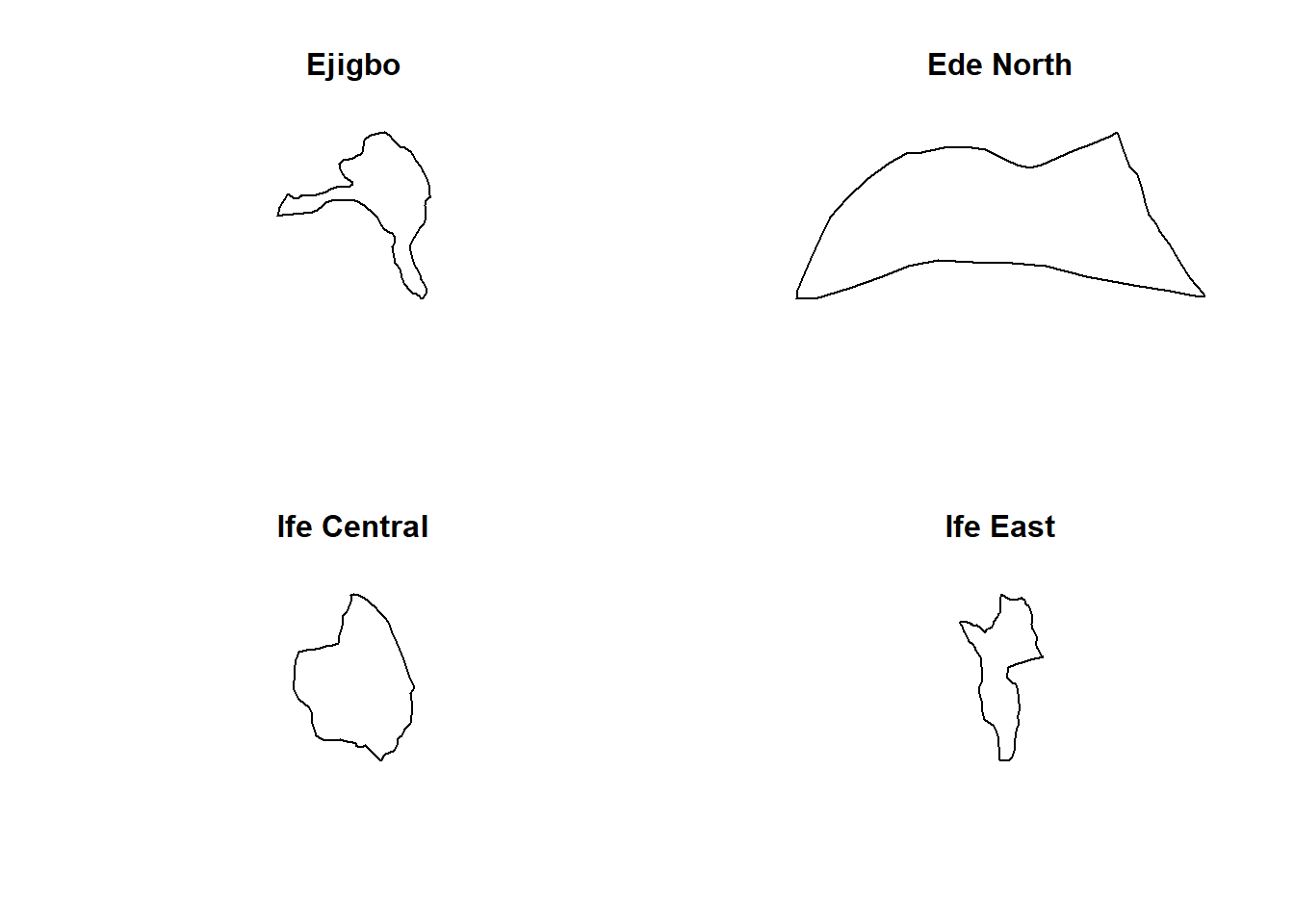
Like before, we need to convert them into owin objects.
ejigbo_owin <- ejigbo %>%
as('Spatial') %>%
as('SpatialPolygons') %>%
as('owin')
ede_north_owin <- ede_north %>%
as('Spatial') %>%
as('SpatialPolygons') %>%
as('owin')
ife_central_owin <- ife_central %>%
as('Spatial') %>%
as('SpatialPolygons') %>%
as('owin')
ife_east_owin <- ife_east %>%
as('Spatial') %>%
as('SpatialPolygons') %>%
as('owin')Next, we need to combine the water point data with the owin objects.
wp_ejigbo_ppp <- func_ppp[ejigbo_owin]
wp_ede_north_ppp <- func_ppp[ede_north_owin]
wp_ife_central_ppp <- non_func_ppp[ife_central_owin]
wp_ife_east_ppp <- non_func_ppp[ife_east_owin]Let’s visualise the combined data!
plot(wp_ejigbo_ppp, main = "Ejigbo")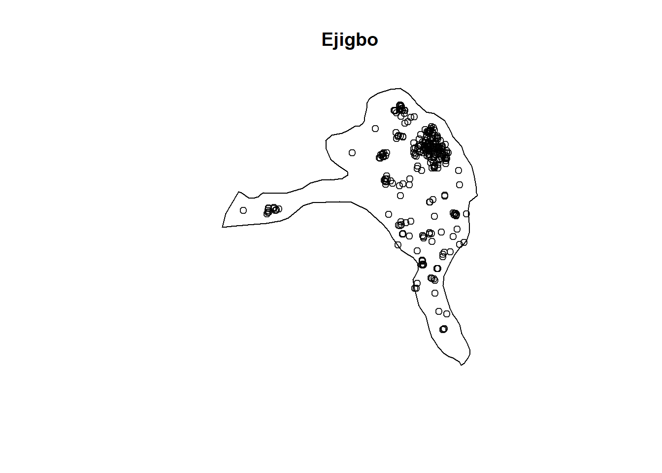
plot(wp_ede_north_ppp, main = "Ede North")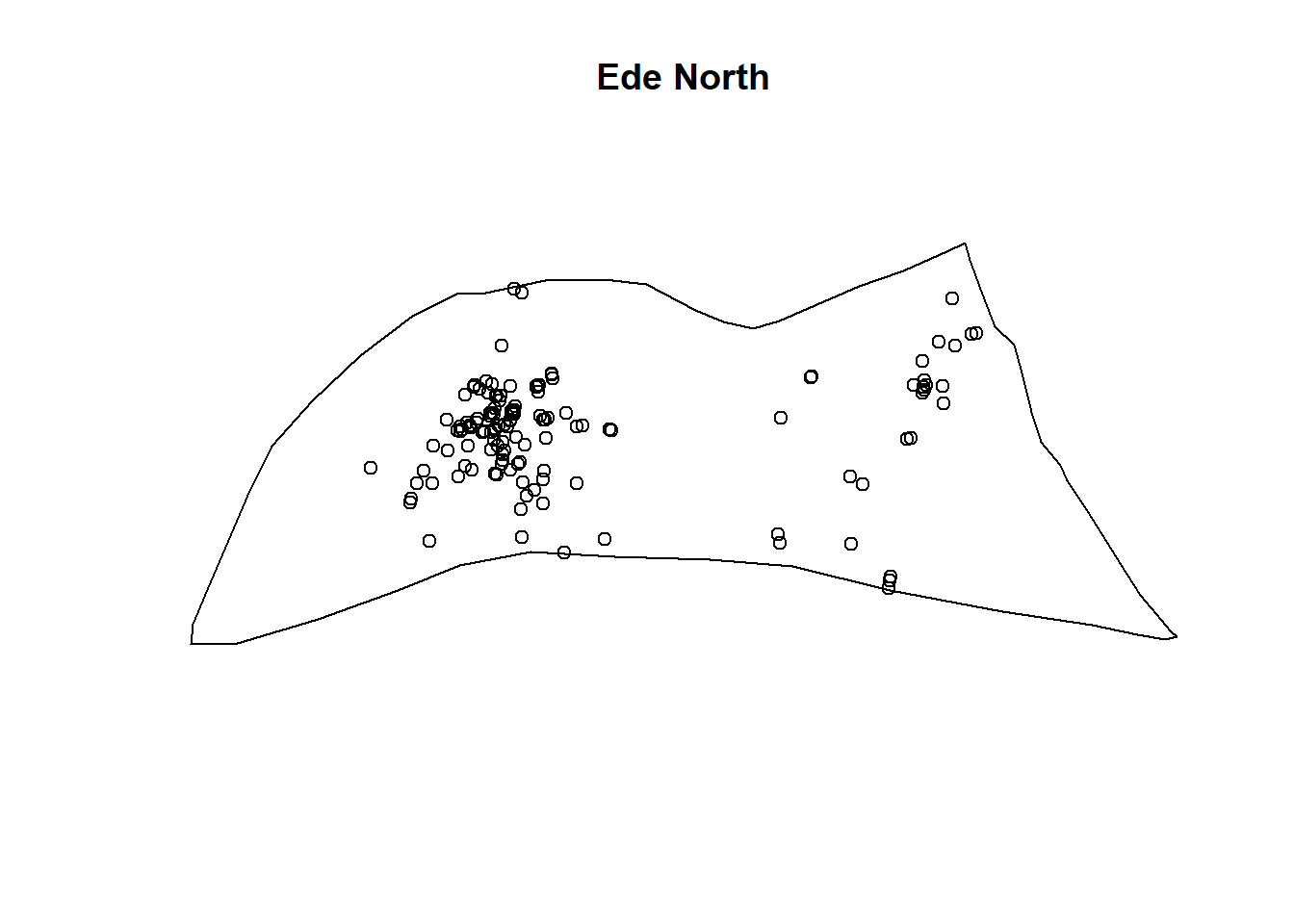
plot(wp_ife_central_ppp, main = "Ife Central")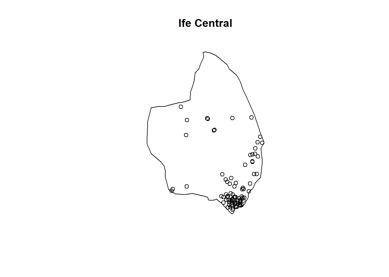
plot(wp_ife_east_ppp, main = "Ife East")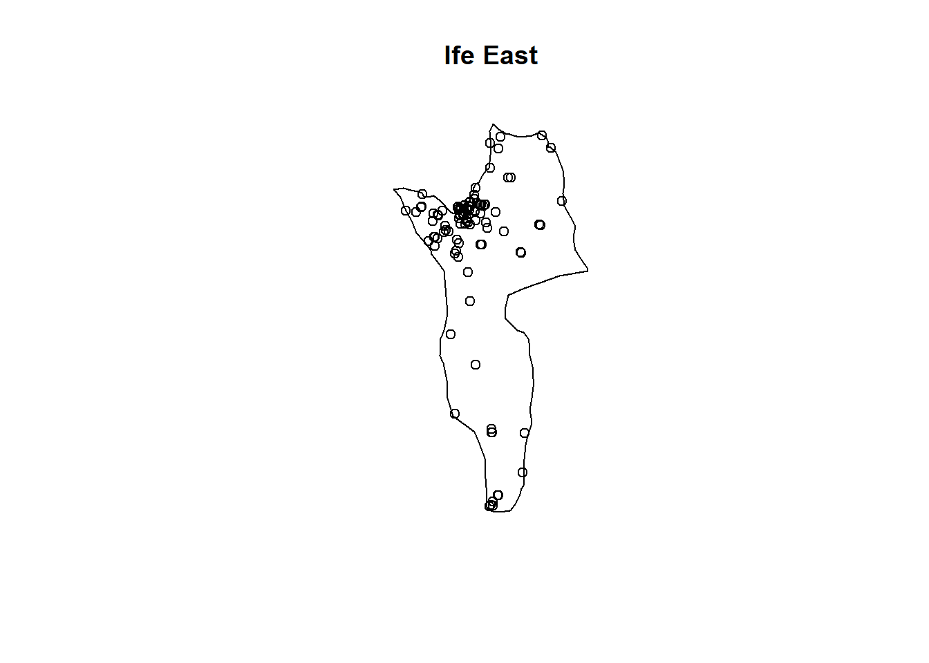
G-Function Complete Spatial Randomness Test
The G-Function measures the distribution of the distances from an arbitrary event to its nearest event. We will be using the spatstat package for this analysis: specifically, the Gest() function to compute G-Function estimation and perform Monte Carlo simulation tests using the envelope() function.
For each Monte Carlo test, we choose to do 39 simulations in accordance to how the envelope() function calculates its significance, where alpha = 2 * nrank / (1 + nsim) by its default pointwise method. Since our alpha is set to 0.05 and nrank is 1 by default, we take nsim = 39.
Functional Water Points
Ejigbo
Compute the G-Function estimate
G_ejigbo <- Gest(wp_ejigbo_ppp, correction = "border")
plot(G_ejigbo, main = "Ejigbo G-Function")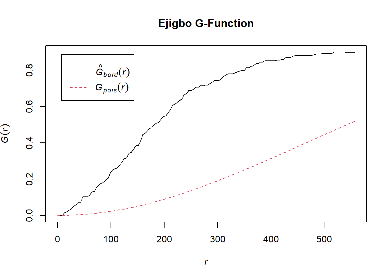
Perform Complete Spatial Randomness Test
G_ejigbo.csr <- envelope(wp_ejigbo_ppp, Gest, nsim=39)Generating 39 simulations of CSR ...
1, 2, 3, 4, 5, 6, 7, 8, 9, 10, 11, 12, 13, 14, 15, 16, 17, 18, 19, 20, 21, 22, 23, 24, 25, 26, 27, 28, 29, 30, 31, 32, 33, 34, 35, 36, 37, 38, 39.
Done.plot(G_ejigbo.csr, main="CSR Ejigbo G-Function")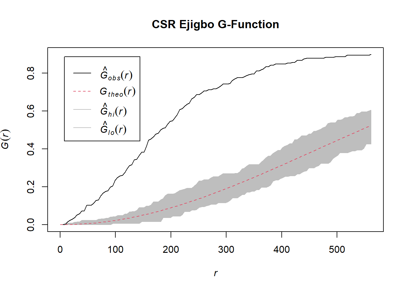
We can observe from the plot that the computed G-function values lie above the envelope, indicating some clustering. Therefore, we can reject the null hypothesis that functional water points in Ejigbo are randomly distributed at 95% confidence interval.
Ede North
Compute the G-Function estimate
G_ede_north <- Gest(wp_ede_north_ppp, correction = "border")
plot(G_ede_north, main = "Ede North G-Function")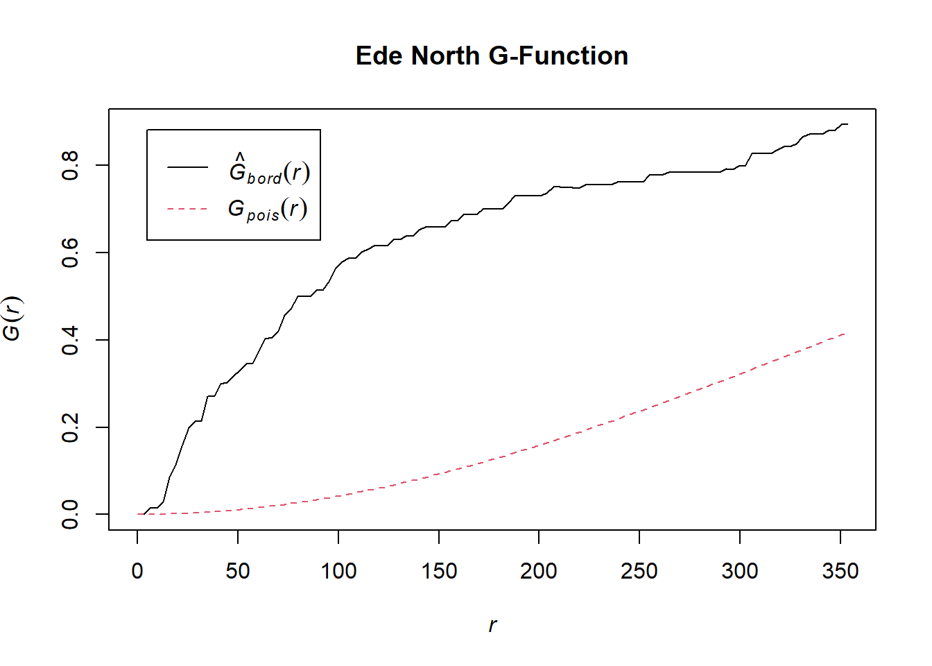
Perform Complete Spatial Randomness Test
G_ede_north.csr <- envelope(wp_ede_north_ppp, Gest, nsim=39)Generating 39 simulations of CSR ...
1, 2, 3, 4, 5, 6, 7, 8, 9, 10, 11, 12, 13, 14, 15, 16, 17, 18, 19, 20, 21, 22, 23, 24, 25, 26, 27, 28, 29, 30, 31, 32, 33, 34, 35, 36, 37, 38, 39.
Done.plot(G_ejigbo.csr, main="CSR Ede North G-Function")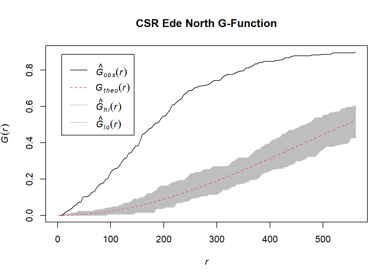
We can observe from the plot that the computed G-function values lie above the envelope, indicating some clustering. Therefore, we can reject the null hypothesis that functional water points in Ede North are randomly distributed at 95% confidence interval.
Non-Functional Water Points
Ife Central
Compute the G-Function estimate
G_ife_central <- Gest(wp_ife_central_ppp, correction = "border")
plot(G_ife_central, main = "Ife Central G-Function")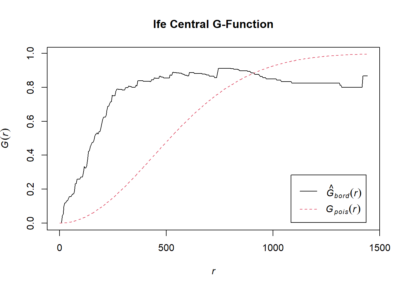
Perform Complete Spatial Randomness Test
G_ife_central.csr <- envelope(wp_ife_central_ppp, Gest, nsim=39)Generating 39 simulations of CSR ...
1, 2, 3, 4, 5, 6, 7, 8, 9, 10, 11, 12, 13, 14, 15, 16, 17, 18, 19, 20, 21, 22, 23, 24, 25, 26, 27, 28, 29, 30, 31, 32, 33, 34, 35, 36, 37, 38, 39.
Done.plot(G_ife_central.csr, main="CSR Ife Central G-Function")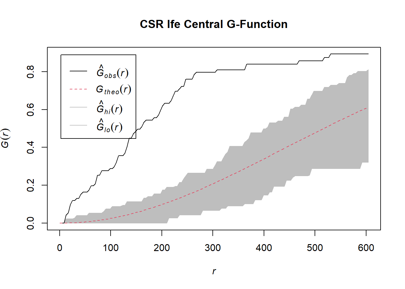
We can observe from the plot that the computed G-function values lie above the envelope, indicating some clustering. Therefore, we can reject the null hypothesis that non-functional water points in Ife Central are randomly distributed at 95% confidence interval.
Ife East
Compute the G-Function estimate
G_ife_central <- Gest(wp_ife_east_ppp, correction = "border")
plot(G_ife_central, main = "Ife East G-Function")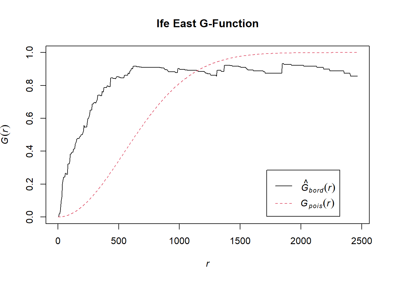
Perform Complete Spatial Randomness Test
G_ife_central.csr <- envelope(wp_ife_east_ppp, Gest, nsim=39)Generating 39 simulations of CSR ...
1, 2, 3, 4, 5, 6, 7, 8, 9, 10, 11, 12, 13, 14, 15, 16, 17, 18, 19, 20, 21, 22, 23, 24, 25, 26, 27, 28, 29, 30, 31, 32, 33, 34, 35, 36, 37, 38, 39.
Done.plot(G_ife_central.csr, main="CSR Ife East G-Function")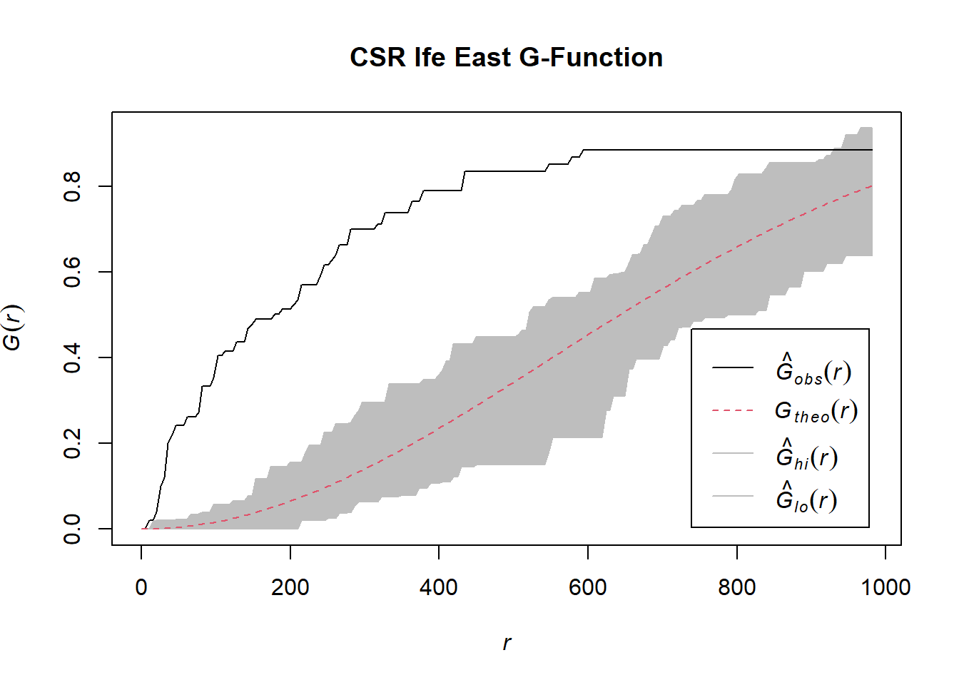
We can observe from the plot that the computed G-function values lie above the envelope, indicating some clustering, except for the r=900 (approximate)-1000 interval. Therefore, for r values below 900, we can reject the null hypothesis that non-functional water points in Ife East are randomly distributed at 95% confidence interval.
Spatial Correlation Analysis
From the Exploratory Data Analysis, we can observe that the water points seem to be concentrated around certain locations. As such, there also seems to be a co-location between the functional and non-functional water points’ distribution, as they are located around the same locations but with their density being seemingly inversely proportional to each other. However, we need to statistically confirm this.
As such, we will be computing the Local Co-Location Quotients (LCLQ) between functional water points and non-functional water points.
H0: Functional water points are not co-located with non-functional water points.
H1: Functional water points are co-located with non-functional water points.
Significance level: 0.05
Extracting categories
We can select a subset of our data containing only Functional and Non-Functional water points. This is because we cannot be certain about the status of Unknown water points, so we do not want them to count towards the computation of the LCLQ.
wp_sf_osun_known <- wp_sf_osun %>%
filter(`func_status` %in% c("Functional", "Non-Functional"))Then, we will extract the functional and non-functional points into vectors.
functional_list <- wp_sf_osun_known %>%
filter(`func_status` == "Functional") %>%
dplyr::pull(`func_status`)
non_functional_list <- wp_sf_osun_known %>%
filter(`func_status` == "Non-Functional") %>%
dplyr::pull(`func_status`)Calculate Local Co-Location Quotient (LCLQ)
To calculate the LCLQ, we need to do several steps.
1) Calculate the k-nearest neighbor
We choose 6 nearest neighbors, but include the point of interest itself (hence ending up with the odd number of 7).
nb <- include_self(st_knn(st_geometry(wp_sf_osun_known), 6))2) Calculate weight matrix
According to the documentation for sfdep’s local_colocation, Wang et. al (2017) emphasises on the use of Gaussian adaptive kernel. Hence, that is what we will be using to compute the weight matrix.
wt <- st_kernel_weights(nb, wp_sf_osun_known, "gaussian", adaptive=TRUE)3) Derive co-location quotient
Using the sfdep function local_colocation(), we calculate the LCLQ for the functional water points.
LCLQ <- local_colocation(functional_list,
non_functional_list,
nb,
wt,
49)After deriving the LCLQ, we combine them into the original dataframe consisting of water point data using the cbind() function of base R.
LCLQ_osun <- cbind(wp_sf_osun_known, LCLQ)We also remove the LCLQ for those that fall above the designated significance level, which is 0.05, as they are not statistically significant.
LCLQ_osun <- LCLQ_osun %>%
mutate(
`p_sim_Non.Functional` = replace(`p_sim_Non.Functional`, `p_sim_Non.Functional` > 0.05, NA),
`Non.Functional` = ifelse(`p_sim_Non.Functional` > 0.05, NA, `Non.Functional`))Analysis
Plotting
tmap_mode("view")
LCLQ_osun <- LCLQ_osun %>% mutate(`size` = ifelse(is.na(`Non.Functional`), 1, 5))
tm_view(set.zoom.limits=c(9, 15),
bbox = st_bbox(filter(LCLQ_osun, !is.na(`Non.Functional`)))) +
tm_shape(osun) +
tm_borders() +
tm_shape(LCLQ_osun) +
tm_dots(col="Non.Functional",
palette=c("cyan", "grey"),
size = "size",
scale=0.15,
border.col = "black",
border.lwd = 0.5,
alpha=0.5,
title="LCLQ"
)tmap_mode("plot")The plot above displays water points with statistically significant LCLQ (i.e. p-value < 0.05). As we can observe, the calculated LCLQ is just under 1. This implies that while the functional water points are isolated (i.e. it is less likely to have non-functional water points within its neighbourhood), the proportion of categories within their neighbourhood is a good representation of the proportion of categories throughout Osun.
Examining colocation using Ripley’s Cross-K (Cross-L) Function
The simulation-based Local Co-location Quotient (LCLQ) proposed by Wang et al. (2017) takes into account that spatial associations vary locally across different spaces. However, traditionally, colocation is measured by Ripley’s Cross-K Function - a modification of Ripley’s K-Function. Unlike the LCLQ, it is a global measure. As such, there is merit in conducting analysis using the Cross-K Function to compare the results against the LCLQ.
For this project, instead of the traditional Cross-K Function, we will be using the normalised version: Cross-L Function. Much like in the Second-order Spatial Points Patterns Analysis, we will be using spatstat’s Lcross() function to compute the value and envelope() to perform the Monte Carlo simulation tests.
We will be operating on the same H0, H1, and significance level as the LCLQ.
Assigning marks to the ppp object
We will be using creating a multitype version of our wp_ppp object that we have created in the Data Preprocessing section, and combining it with the osun_owin object. However, for the purpose of computing the L-Cross Function, we need to assign marks to the ppp object - specifically denoting the func_status.
wp_ppp_marked <- wp_ppp
marks(wp_ppp_marked) <- factor(wp_sf_osun$func_status)
wp_osun_ppp_marked = wp_ppp_marked[osun_owin]We can now see that the points are categorised based on their func_status.
plot(wp_osun_ppp_marked)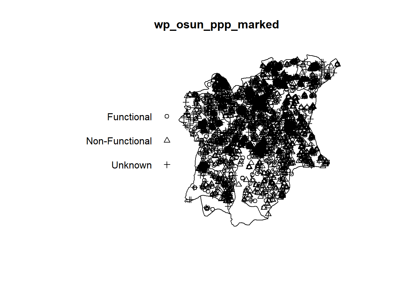
Again, however, we need to rescale the data to km.
wp_osun_ppp_marked.km <- rescale(wp_osun_ppp_marked, 1000, "km")Computing Cross-L Function
wp_osun_Lcross.csr <- envelope(wp_osun_ppp_marked.km,
Lcross,
i="Functional",
j="Non-Functional",
correction="border",
nsim=39)Generating 39 simulations of CSR ...
1, 2, 3, 4, 5, 6, 7, 8, 9, 10, 11, 12, 13, 14, 15, 16, 17, 18, 19, 20, 21, 22, 23, 24, 25, 26, 27, 28, 29, 30, 31, 32, 33, 34, 35, 36, 37, 38, 39.
Done.plot(wp_osun_Lcross.csr, xlim=c(0,10), main="L-Cross Function", legend=FALSE)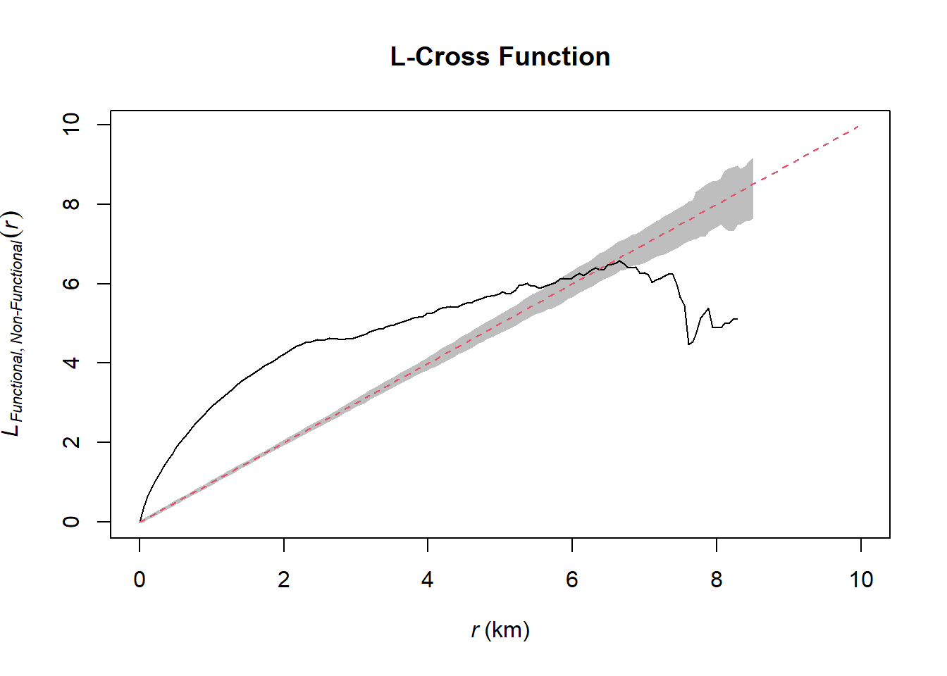
We can see that from distances 0 - slightly before 6 km (approximate) there seems to be clustering between the functional and non-functional water points. However, from 7 km onwards (approximate), there seems to be dispersion instead. For those intervals, we can reject the null hypothesis that functional water points and non-functional water points are independently distributed at 95% confidence interval.